Introduction to Custom Contrasts
Custom contrasts transform statistical analysis from exploratory to confirmatory. Instead of asking "do these groups differ?", you ask precise questions like "does performance increase linearly with dosage?" or "do the extreme groups differ from the middle group?"
What You'll Master
- Design theory-driven contrasts for specific hypotheses
- Apply polynomial contrasts for trend analysis
- Create custom contrast weights for complex comparisons
- Understand and manage multiple testing issues
- Interpret effect sizes for contrast-specific questions
- Distinguish planned vs post-hoc comparisons
- Apply contrasts to dose-response and trend analysis
- Completed the emmeans interpretation tutorial
- Understanding of hypothesis testing and p-values
- Familiarity with linear combinations and weighted averages
- Same packages:
tidyverse,glmmTMB,emmeans
Polynomial Trends: Testing for Patterns
Polynomial contrasts test whether responses follow linear, quadratic, or higher-order trends across ordered groups. This is especially valuable for dose-response studies, developmental research, or any situation with naturally ordered categories.
# Set up analysis with ordered performance categories
library(tidyverse)
library(glmmTMB)
library(emmeans)

data(mtcars)

# Create ordered performance categories
mtcars_enhanced <- mtcars %>%
  mutate(
    hp_category = cut(hp, breaks = c(0, 120, 200, Inf),
                      labels = c("Economy", "Standard", "Performance")),
    cyl_category = factor(cyl, levels = c(4, 6, 8),
                         labels = c("Four", "Six", "Eight"))
  )

# Check sample balance
table(mtcars_enhanced$hp_category)

# Fit model for trend analysis
model_hp <- glmmTMB(mpg ~ hp_category, data = mtcars_enhanced)
hp_emmeans <- emmeans(model_hp, ~ hp_category)

# Test polynomial trends
hp_trends <- contrast(hp_emmeans, "poly")
print(hp_trends)| Trend Component | Estimate | SE | p-value | Interpretation |
|---|---|---|---|---|
| Linear | -11.57 | 1.43 | < 0.001 | Strong linear decrease |
| Quadratic | 3.56 | 2.76 | 0.198 | No curvature detected |
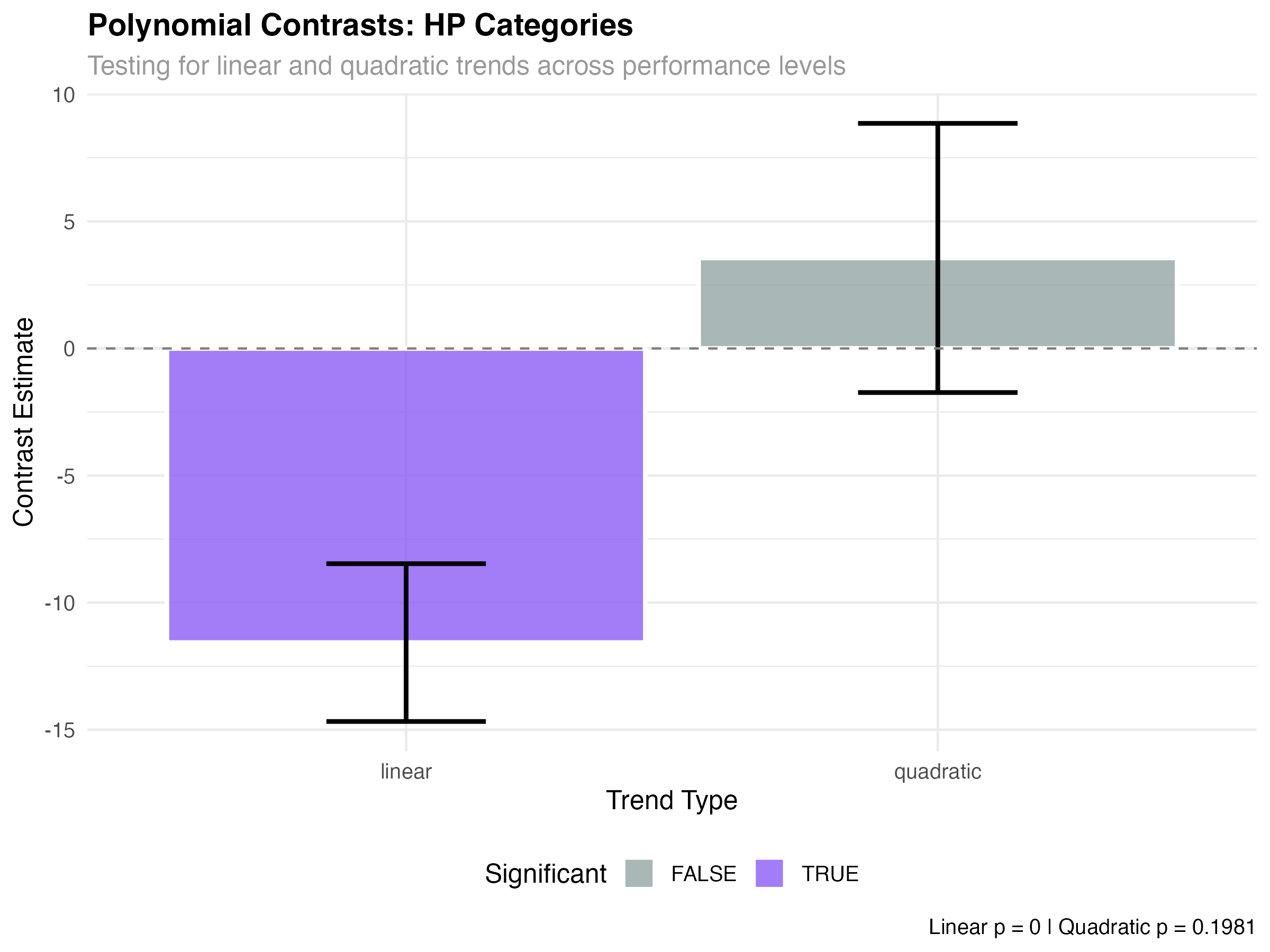
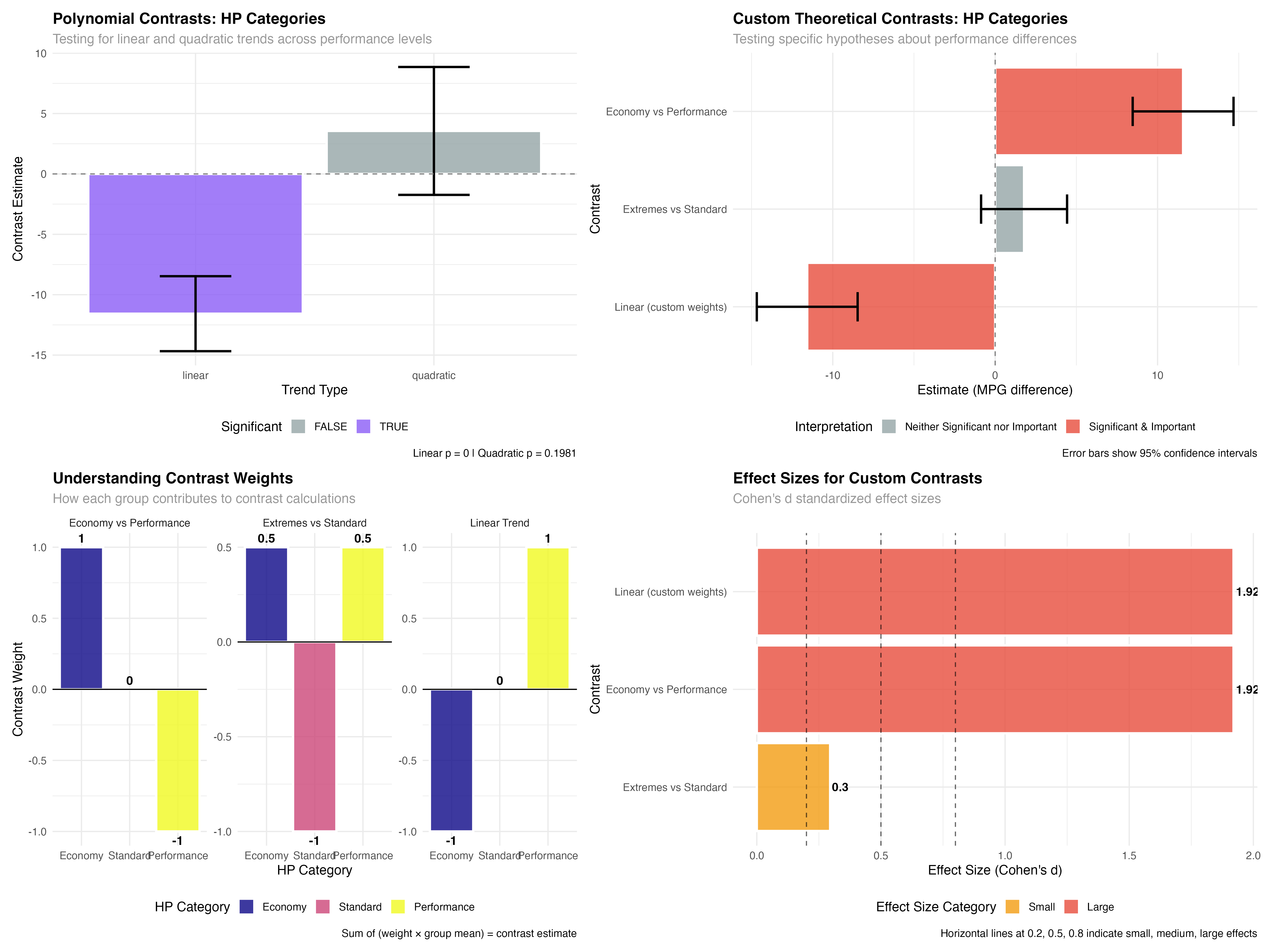
- Significant linear trend (p < 0.001): Fuel efficiency decreases consistently across performance levels
- Non-significant quadratic (p = 0.198): The relationship is purely linear - no acceleration or deceleration
- Effect size: 11.6 MPG difference from Economy to Performance represents a large practical effect
Dose-Response Analysis with Cylinders
# Analyze cylinder count as ordered "doses"
model_cyl <- glmmTMB(mpg ~ cyl_category, data = mtcars_enhanced)
cyl_emmeans <- emmeans(model_cyl, ~ cyl_category)

# Test for dose-response patterns
cyl_trends <- contrast(cyl_emmeans, "poly")
print(cyl_trends)

# Calculate means for visualization
cyl_means <- as.data.frame(cyl_emmeans)
print(cyl_means)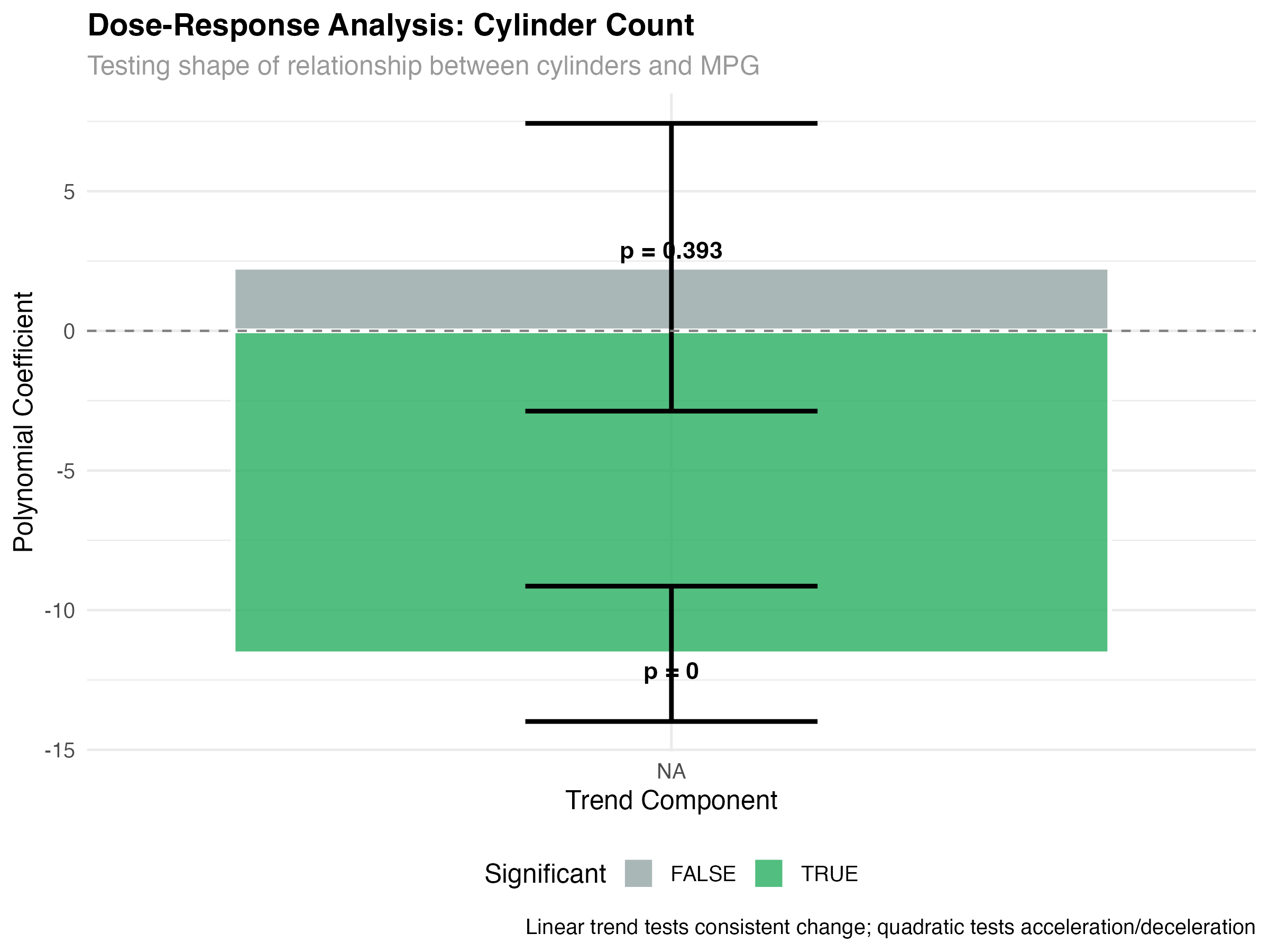
= ~5.8 MPG penalty per cylinder pair
Custom Theory-Driven Contrasts
The real power of contrasts lies in testing specific theories. Rather than using pre-built contrast families, you design weights that directly test your hypotheses.
- Theory 1: Economy cars vs Performance cars (ignoring Standard)
- Theory 2: Standard cars vs the average of extreme categories
- Theory 3: Linear progression across all three categories
# Design custom theoretical contrasts
custom_contrasts <- list(
  "Economy vs Performance" = c(1, 0, -1),      # Compare extremes only
  "Extremes vs Standard" = c(0.5, -1, 0.5),    # Standard vs average of extremes
  "Linear (custom weights)" = c(-1, 0, 1)      # Custom linear progression
)

# Apply custom contrasts
hp_custom <- contrast(hp_emmeans, custom_contrasts)
custom_results <- as.data.frame(hp_custom) %>%
  mutate(
    significant = p.value < 0.05,
    effect_size = abs(estimate) / sqrt(var(mtcars$mpg)),
    practical_importance = abs(estimate) > 3,  # 3+ MPG threshold
    interpretation = case_when(
      significant & practical_importance ~ "Significant & Important",
      significant & !practical_importance ~ "Significant but Small",
      !significant & practical_importance ~ "Large but Uncertain",
      TRUE ~ "Neither Significant nor Important"
    )
  )

print(custom_results[, c("contrast", "estimate", "p.value", "interpretation")])| Custom Contrast | Estimate | p-value | Interpretation |
|---|---|---|---|
| Economy vs Performance | 11.57 | < 0.001 | Significant & Important |
| Extremes vs Standard | 1.78 | 0.198 | Neither Significant nor Important |
| Linear (custom weights) | -11.57 | < 0.001 | Significant & Important |
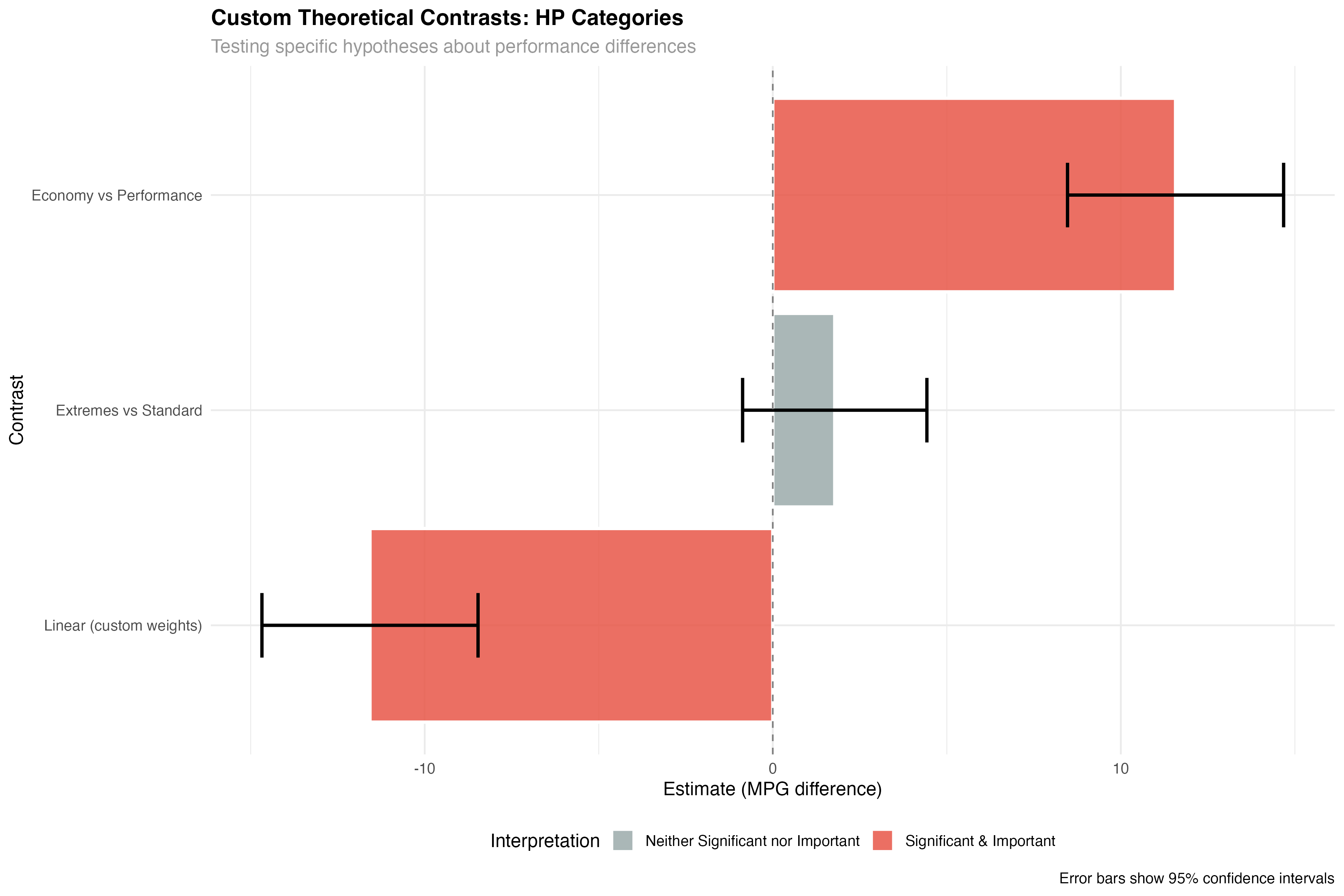
- Theory 1 supported: Economy cars significantly outperform Performance cars by 11.6 MPG
- Theory 2 unsupported: Standard cars don't differ significantly from the average of extremes
- Theory 3 supported: Strong linear progression confirms dose-response relationship
Planned vs Exploratory Comparisons
# Compare planned contrasts vs pairwise comparisons
hp_pairwise <- pairs(hp_emmeans)
pairwise_results <- as.data.frame(hp_pairwise)

# Show the difference in approach
cat("Planned contrasts test specific theories:\n")
print(custom_results[, c("contrast", "estimate", "p.value")])

cat("\nPairwise comparisons test all possible differences:\n")
print(pairwise_results[, c("contrast", "estimate", "p.value")])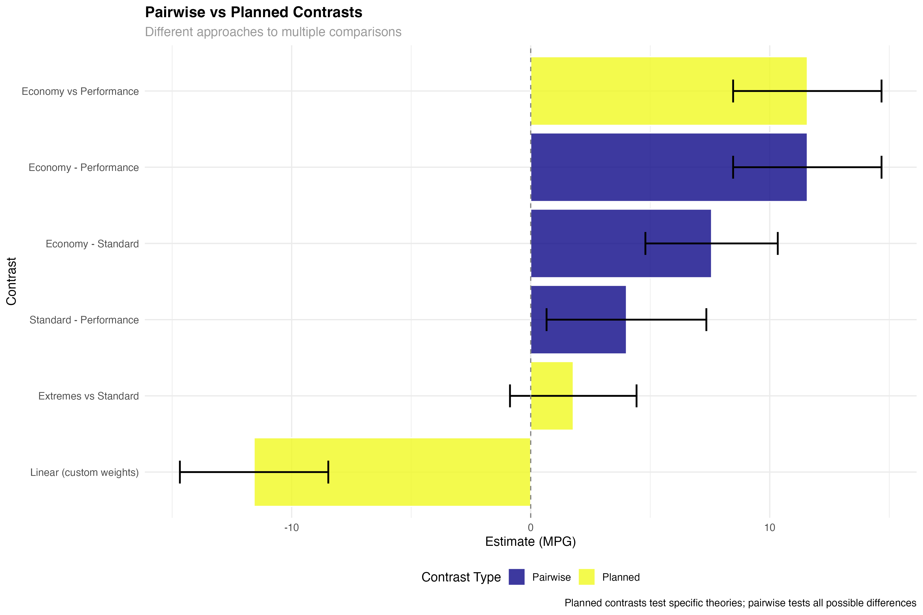
Understanding Contrast Weights
Contrast weights determine how each group contributes to the comparison. Understanding how to design and interpret these weights is crucial for creating meaningful contrasts.
# Visualize how contrast weights work
hp_means <- as.data.frame(hp_emmeans)

# Create data showing weight contributions
weight_examples <- data.frame(
  hp_category = rep(hp_means$hp_category, 3),
  contrast_name = rep(c("Economy vs Performance", "Extremes vs Standard", "Linear Trend"),
                     each = 3),
  weight = c(1, 0, -1,      # Economy vs Performance
            0.5, -1, 0.5,   # Extremes vs Standard
            -1, 0, 1),      # Linear Trend
  group_mean = rep(hp_means$emmean, 3)
) %>%
  mutate(
    contribution = weight * group_mean,
    contrast_estimate = rep(c(
      sum(c(1, 0, -1) * hp_means$emmean),           # Economy vs Performance
      sum(c(0.5, -1, 0.5) * hp_means$emmean),      # Extremes vs Standard
      sum(c(-1, 0, 1) * hp_means$emmean)           # Linear Trend
    ), each = 3)
  )

print("Weight contributions for each contrast:")
print(weight_examples)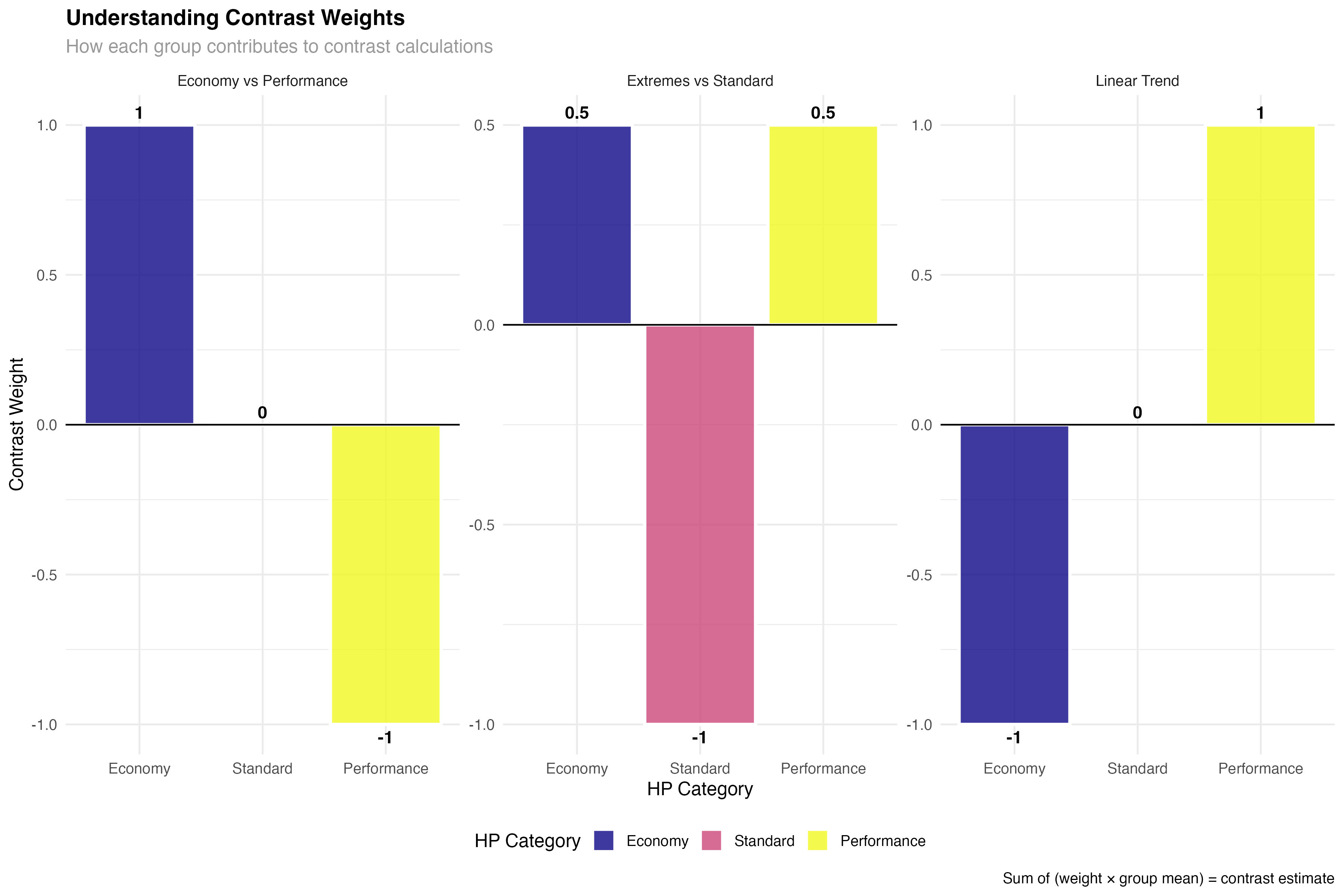
- Positive weights: Groups that contribute positively to the contrast
- Negative weights: Groups that are subtracted in the comparison
- Zero weights: Groups ignored in this specific contrast
- Sum constraint: Weights must sum to zero for valid contrasts
- Equal weighting: Use equal absolute values when groups should contribute equally
Designing Meaningful Weights
- Theory-driven: Weights should reflect your specific research hypothesis
- Interpretable: Use simple fractions (0.5, -1, 0.5) rather than complex decimals
- Balanced: Consider sample sizes when groups have very different n's
- Orthogonal: Independent contrasts should test different aspects of your data
- Drug effect: [-1, 0.5, 0.5] tests any drug vs placebo
- Dose response: [0, -1, 1] tests low vs high dose
- Linear trend: [-1, 0, 1] tests for linear dose-response
Multiple Testing Considerations
When testing multiple contrasts, you need to control the family-wise error rate. Different adjustment methods have different trade-offs between Type I and Type II error protection.
# Compare different multiple testing adjustments
unadjusted_p <- custom_results$p.value
bonferroni_p <- p.adjust(custom_results$p.value, method = "bonferroni")
holm_p <- p.adjust(custom_results$p.value, method = "holm")
fdr_p <- p.adjust(custom_results$p.value, method = "fdr")

# Create comparison table
adjustment_comparison <- data.frame(
  Contrast = custom_results$contrast,
  Unadjusted = round(unadjusted_p, 4),
  Bonferroni = round(bonferroni_p, 4),
  Holm = round(holm_p, 4),
  FDR = round(fdr_p, 4)
)

print("P-value adjustments for multiple contrasts:")
print(adjustment_comparison)

# Test effects of different adjustments on significance
sig_comparison <- adjustment_comparison %>%
  mutate(
    Sig_Unadjusted = Unadjusted < 0.05,
    Sig_Bonferroni = Bonferroni < 0.05,
    Sig_Holm = Holm < 0.05,
    Sig_FDR = FDR < 0.05
  )

print("Significance under different adjustment methods:")
print(sig_comparison[, c("Contrast", "Sig_Unadjusted", "Sig_Bonferroni", "Sig_Holm", "Sig_FDR")])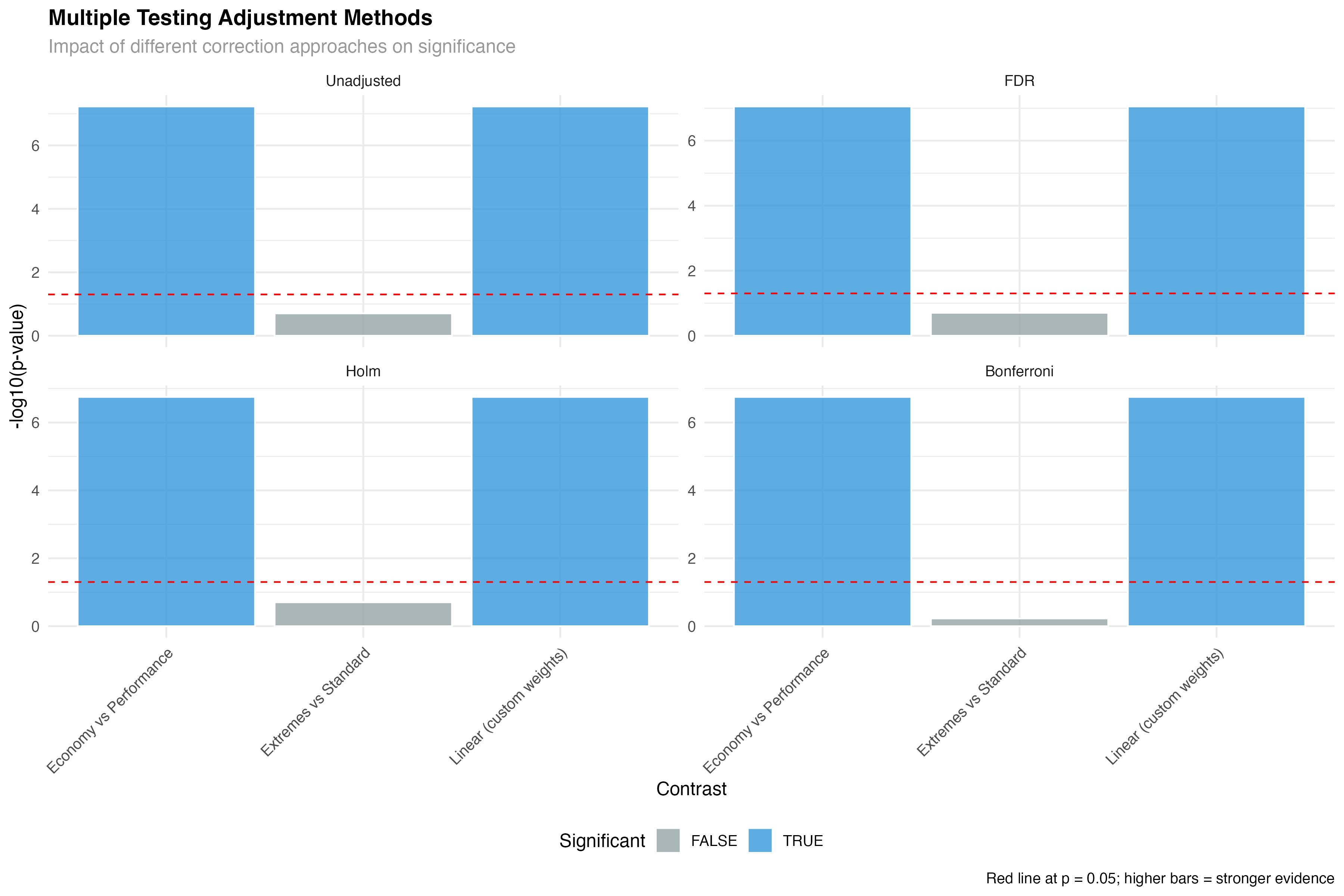
- Bonferroni: Most conservative, controls family-wise error rate strictly
- Holm: Less conservative than Bonferroni but still controls FWER
- FDR (Benjamini-Hochberg): Controls false discovery rate, more power
- Unadjusted: Appropriate for small numbers of planned, orthogonal contrasts
Effect Sizes for Contrasts
Statistical significance tells you if an effect exists; effect sizes tell you if it matters practically. For contrasts, effect sizes help you understand the magnitude of specific comparisons.
# Calculate standardized effect sizes for contrasts
effect_size_data <- custom_results %>%
  mutate(
    # Cohen's d approximation for contrasts
    cohens_d = abs(estimate) / sqrt(var(mtcars$mpg)),
    # Classify effect magnitude
    effect_category = case_when(
      cohens_d < 0.2 ~ "Negligible",
      cohens_d < 0.5 ~ "Small",
      cohens_d < 0.8 ~ "Medium",
      TRUE ~ "Large"
    ) %>% factor(levels = c("Negligible", "Small", "Medium", "Large")),
    # Practical significance threshold (3 MPG difference)
    practically_significant = abs(estimate) > 3
  )

print("Effect sizes for custom contrasts:")
print(effect_size_data[, c("contrast", "estimate", "cohens_d", "effect_category")])| Contrast | Estimate (MPG) | Cohen's d | Effect Category | Practical Significance |
|---|---|---|---|---|
| Economy vs Performance | 11.57 | 1.92 | Large | Yes (>3 MPG) |
| Extremes vs Standard | 1.78 | 0.30 | Small | No (<3 MPG) |
| Linear (custom weights) | 11.57 | 1.92 | Large | Yes (>3 MPG) |
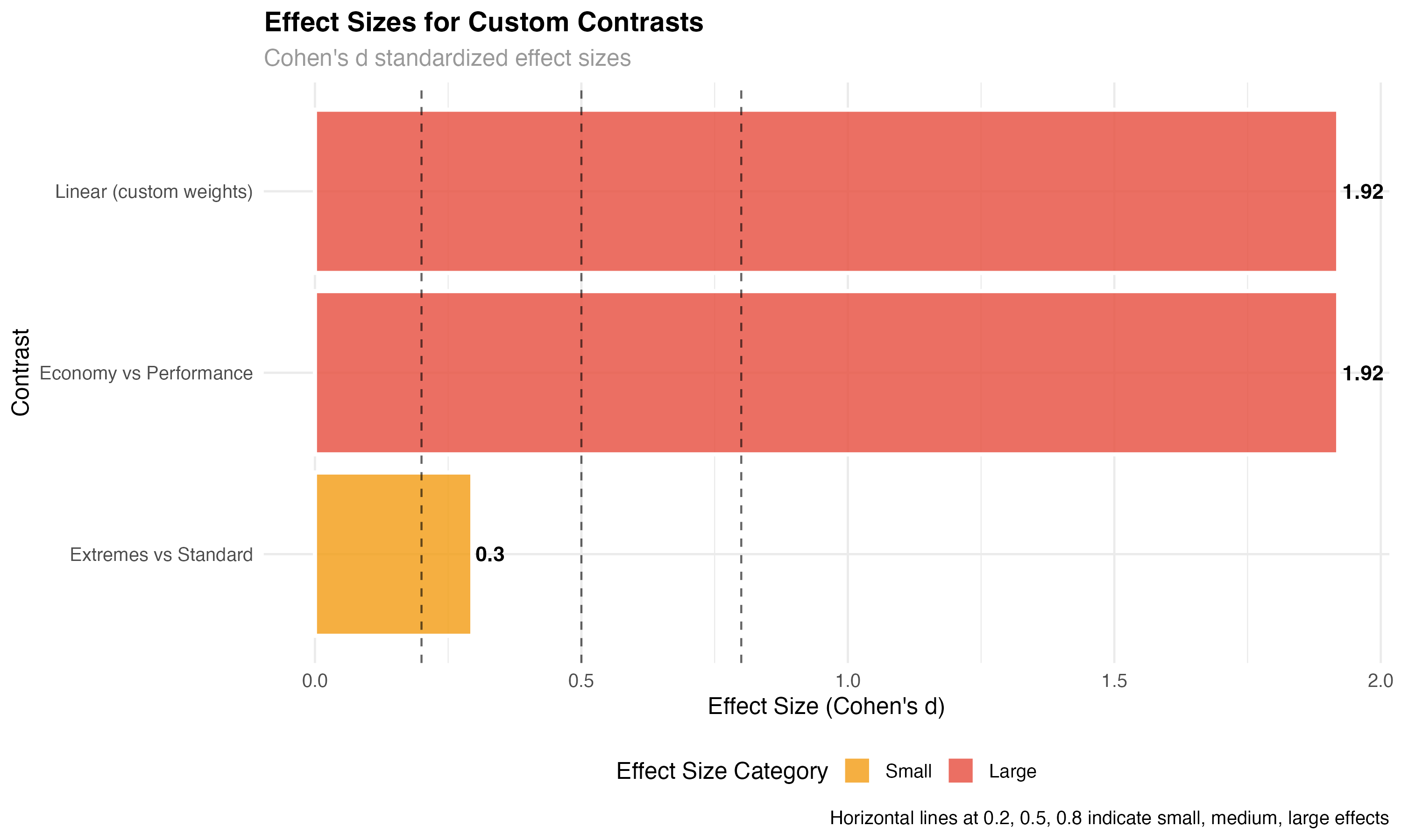
- Economy vs Performance: Large effect (d = 1.92) with high practical significance (11.6 MPG difference)
- Extremes vs Standard: Small effect (d = 0.30) with limited practical importance (1.8 MPG difference)
- Linear trend: Large effect confirming consistent dose-response relationship
Advanced Applications & Best Practices
When to Use Different Contrast Types
| Contrast Type | Best For | Example Application | Key Advantage |
|---|---|---|---|
| Polynomial | Ordered groups, dose-response | Drug dosage effects | Tests specific trend shapes |
| Custom theoretical | A priori hypotheses | Theory testing | High statistical power |
| Helmert | Sequential comparisons | Developmental stages | Each vs all subsequent |
| Treatment vs control | Multiple treatments vs reference | Clinical trials | Controls Type I error |
Complete Analysis Workflow
- ✅ Polynomial trends: Test for linear, quadratic, cubic patterns in ordered data
- ✅ Custom contrasts: Design theory-specific comparisons with meaningful weights
- ✅ Effect size evaluation: Distinguish statistical from practical significance
- ✅ Multiple testing control: Choose appropriate adjustment methods
- ✅ Weight interpretation: Understand what each contrast actually tests
- ✅ Research integration: Connect statistical results to scientific theories
Contrast Design Checklist
- 📝 Define hypotheses first: What specific theory are you testing?
- ⚖️ Check weight constraints: Do weights sum to zero?
- 🎯 Ensure interpretability: Can you explain what each contrast means?
- 🔢 Consider sample sizes: Are groups balanced enough for meaningful comparison?
- 📊 Plan for multiple testing: How many contrasts will you test?
- 🔍 Set practical thresholds: What effect size would be meaningful?
What You've Mastered
✅ Advanced Contrast Skills
- Designing theory-driven contrasts for specific research hypotheses
- Applying polynomial contrasts for trend and dose-response analysis
- Creating and interpreting custom contrast weights
- Managing multiple testing with appropriate correction methods
- Calculating and interpreting effect sizes for contrast-specific questions
- Distinguishing planned from exploratory comparisons
- Integrating contrast results with scientific theory and practical applications
Beyond Contrasts: Future Directions
- Multivariate contrasts: Testing hypotheses across multiple outcomes simultaneously
- Bayesian contrasts: Incorporating prior beliefs and uncertainty quantification
- Machine learning integration: Feature importance as modern contrast analysis
- Causal inference: Contrasts for treatment effect estimation
- Meta-analysis: Combining contrast results across studies
- Robust contrasts: Methods less sensitive to outliers and violations