Estimated Marginal Means in R: Making Complex Models Interpretable

Lesson 5

Introduction to Estimated Marginal Means

You've mastered model fitting, comparison, diagnostics, and validation. Now comes the crucial final step: turning statistical results into clear, actionable insights that stakeholders can understand and use. EMmeans bridges the gap between complex models and practical interpretation.

Estimated marginal means (also called least-squares means) answer the question: "What would the outcome be for typical cases in each group, holding other factors constant?" This is exactly what decision-makers need to know.

What You'll Learn

Calculate marginal means for categorical and continuous predictors
Decompose complex interactions into interpretable simple effects
Perform pairwise comparisons with proper multiple testing corrections
Visualize effects for clear stakeholder communication
Translate statistical significance into practical importance
Handle both categorical and continuous predictors appropriately
Create publication-ready effect summaries

Before You Begin:

Completed the full modeling sequence (fitting through validation)
Understanding of interaction effects and their interpretation
New package: emmeans (install with install.packages("emmeans"))
Familiarity with confidence intervals and statistical significance

The EMmeans Philosophy: Rather than reporting raw model coefficients (which depend on coding schemes), emmeans provides estimates for meaningful, real-world scenarios. Instead of "a 1-unit increase in X leads to β change in Y," you get "high-performance cars average 18.2 MPG (95% CI: 16.1-20.3)."

Step 1

Marginal Means for Categorical Effects

Let's start by converting our continuous predictors into meaningful categories and examining their marginal means. This approach makes results immediately interpretable for practical decision-making.

# Set up emmeans analysis with categorical predictors
library(tidyverse)
library(glmmTMB)
library(emmeans)

data(mtcars)

# Create meaningful categories from continuous variables
mtcars_enhanced <- mtcars %>%
  mutate(
    # Horsepower categories based on car performance
    hp_category = cut(hp, breaks = c(0, 150, 250, Inf), 
                      labels = c("Low", "Medium", "High")),
    # Weight categories based on vehicle class
    wt_category = cut(wt, breaks = c(0, 3.2, 4.2, Inf),
                      labels = c("Light", "Medium", "Heavy"))
  )

# Check sample sizes for balance
table(mtcars_enhanced$hp_category, mtcars_enhanced$wt_category)

# Fit categorical interaction model
model_categorical <- glmmTMB(mpg ~ hp_category * wt_category, data = mtcars_enhanced)

# Calculate estimated marginal means
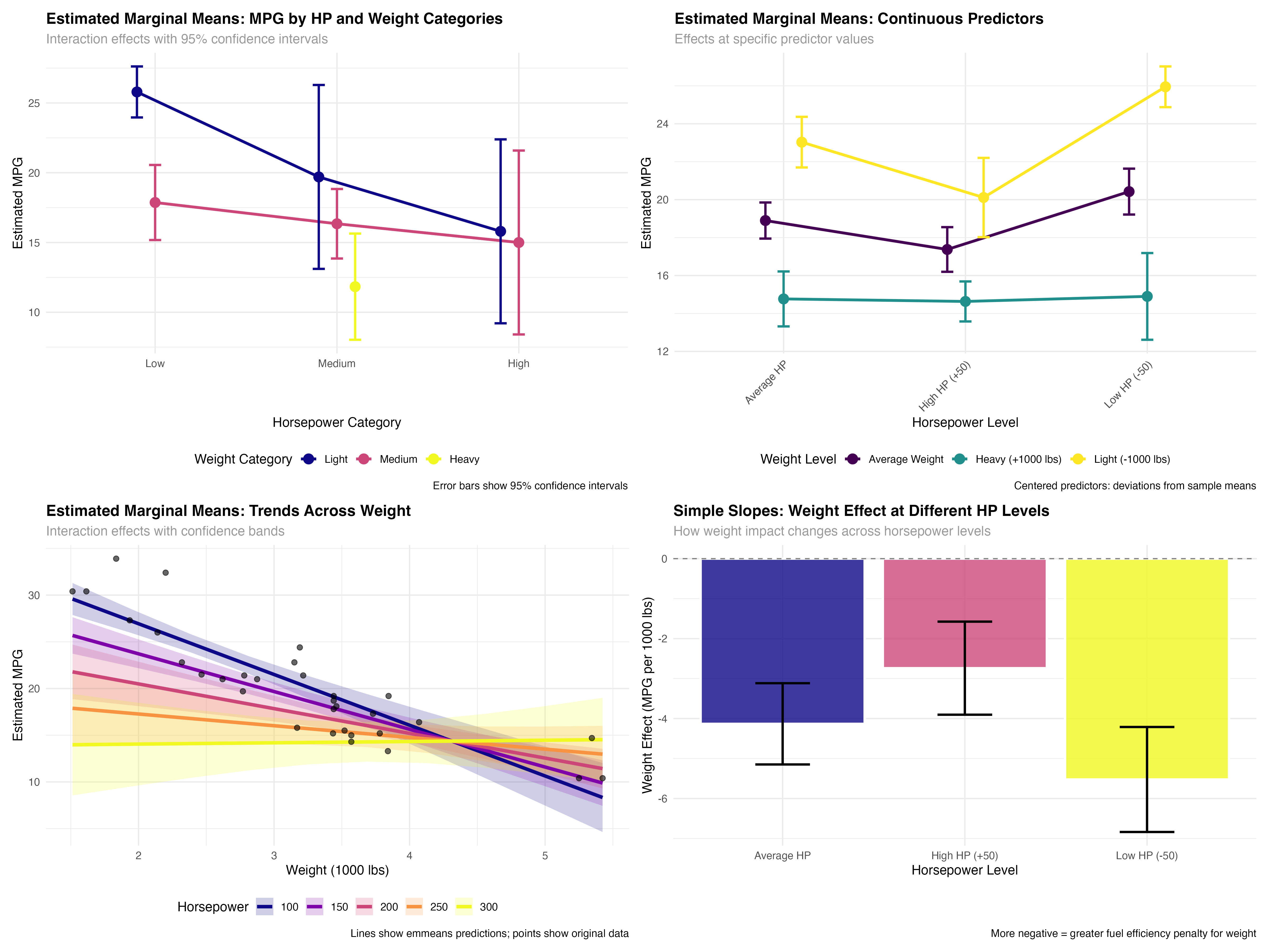
emm_categorical <- emmeans(model_categorical, ~ hp_category * wt_category)
summary(emm_categorical)

HP Category	Weight Category	Estimated MPG	95% CI Lower	95% CI Upper
Low	Light	25.8	24.0	27.6
Medium	Light	19.7	13.1	26.3
High	Light	15.8	9.2	22.4
Low	Medium	17.9	15.2	20.6
Medium	Medium	16.3	13.9	18.8
High	Medium	15.0	8.4	21.6

Estimated Marginal Means by Category

Categorical estimated marginal means with confidence intervals

Key patterns revealed:

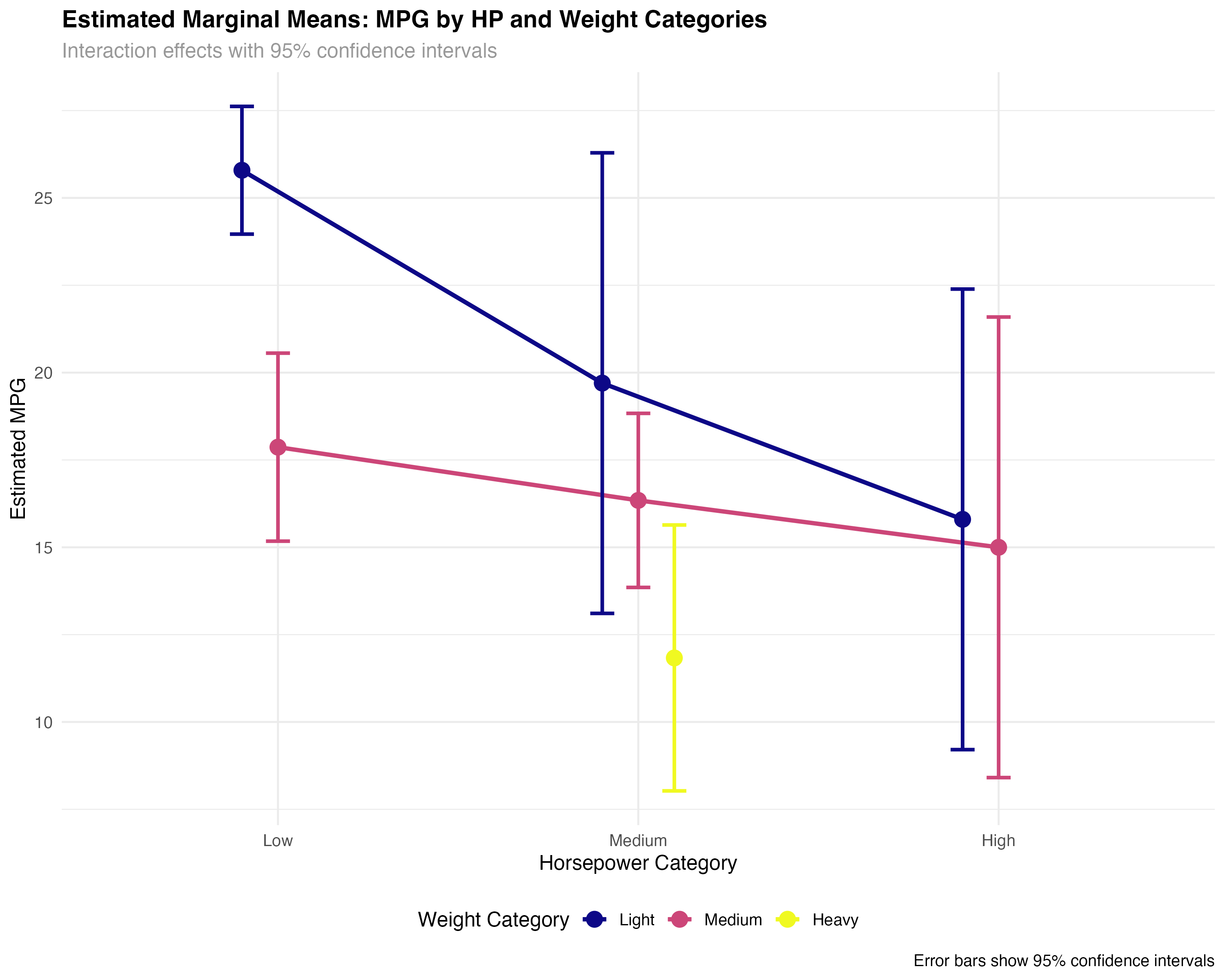
Light, low-HP cars: Best fuel efficiency (25.8 MPG) with tight confidence intervals
Weight penalty varies by HP: Heavy cars show different patterns across horsepower levels
Uncertainty increases: Wider confidence intervals for rare combinations (high-HP light cars)
Missing combinations: Some categories lack sufficient data (heavy, low-HP cars)

Interpreting Categorical Marginal Means

Point estimates: Expected MPG for the "average" car in each category combination
Confidence intervals: Range of plausible values for the true population mean
Non-overlapping CIs: Strong evidence of meaningful differences between groups
Wide intervals: Indicate small sample sizes or high variability within groups

Step 2

Marginal Means for Continuous Predictors

For continuous predictors, emmeans calculates estimates at specific values you choose. This allows you to explore effects at meaningful points like "1 standard deviation below average" or "typical values in your population."

# Work with centered continuous predictors for interpretability
mtcars_enhanced <- mtcars_enhanced %>%
  mutate(
    wt_c = wt - mean(wt),  # Centered weight
    hp_c = hp - mean(hp)   # Centered horsepower
  )

# Fit interaction model with centered predictors
model_interaction <- glmmTMB(mpg ~ wt_c * hp_c, data = mtcars_enhanced)

# Calculate emmeans at meaningful values
# -1, 0, +1 represent light, average, heavy cars
# -50, 0, +50 represent low, average, high horsepower
emm_continuous <- emmeans(model_interaction, ~ wt_c * hp_c, 
                         at = list(wt_c = c(-1, 0, 1), hp_c = c(-50, 0, 50)))

# Display results with meaningful labels
emm_data <- as.data.frame(emm_continuous) %>%
  mutate(
    wt_label = case_when(
      wt_c == -1 ~ "Light (-1000 lbs from avg)",
      wt_c == 0 ~ "Average Weight",
      wt_c == 1 ~ "Heavy (+1000 lbs from avg)"
    ),
    hp_label = case_when(
      hp_c == -50 ~ "Low HP (-50 from avg)",
      hp_c == 0 ~ "Average HP", 
      hp_c == 50 ~ "High HP (+50 from avg)"
    )
  )

print(emm_data[, c("wt_label", "hp_label", "emmean", "lower.CL", "upper.CL")])

Weight Level	HP Level	Estimated MPG	95% CI Lower	95% CI Upper
Light (-1000 lbs)	Low HP (-50)	25.9	24.9	27.0
Average Weight	Low HP (-50)	20.4	19.2	21.6
Heavy (+1000 lbs)	Low HP (-50)	14.9	12.6	17.2
Light (-1000 lbs)	Average HP	23.0	21.7	24.4
Average Weight	Average HP	18.9	17.9	19.8
Heavy (+1000 lbs)	Average HP	14.8	13.3	16.2

Continuous Predictor Marginal Means

Estimated marginal means for continuous predictors at specific values

Continuous predictor insights:

Consistent weight effect: ~5.5 MPG penalty per 1000 lbs across HP levels
HP interaction: High-HP cars show smaller weight penalties than low-HP cars
Precise estimates: Narrow confidence intervals due to continuous predictor precision
Practical ranges: Estimates cover realistic combinations of weight and horsepower

Trend Analysis Across Continuous Range

# Create smooth trends across the full range of weight values
wt_range <- seq(min(mtcars$wt), max(mtcars$wt), length.out = 10)
hp_levels <- c(100, 150, 200, 250, 300)

# Get emmeans predictions across full range
emm_trends <- emmeans(model_interaction, ~ wt_c * hp_c, at = list(
  wt_c = wt_range - mean(mtcars$wt),
  hp_c = hp_levels - mean(mtcars$hp)
))

# Visualize trends with confidence bands
ggplot(trend_data, aes(x = wt_original, y = emmean, color = factor(hp_original))) +
  geom_ribbon(aes(ymin = lower.CL, ymax = upper.CL, fill = factor(hp_original)), 
              alpha = 0.2, color = NA) +
  geom_line(linewidth = 1.5) +
  geom_point(data = mtcars, aes(x = wt, y = mpg), 
             color = "black", size = 2, alpha = 0.6, inherit.aes = FALSE) +
  scale_color_viridis_d(name = "Horsepower") +
  scale_fill_viridis_d(name = "Horsepower") +
  labs(title = "Fuel Efficiency Trends Across Weight Range",
       x = "Weight (1000 lbs)", y = "Estimated MPG") +
  theme_minimal()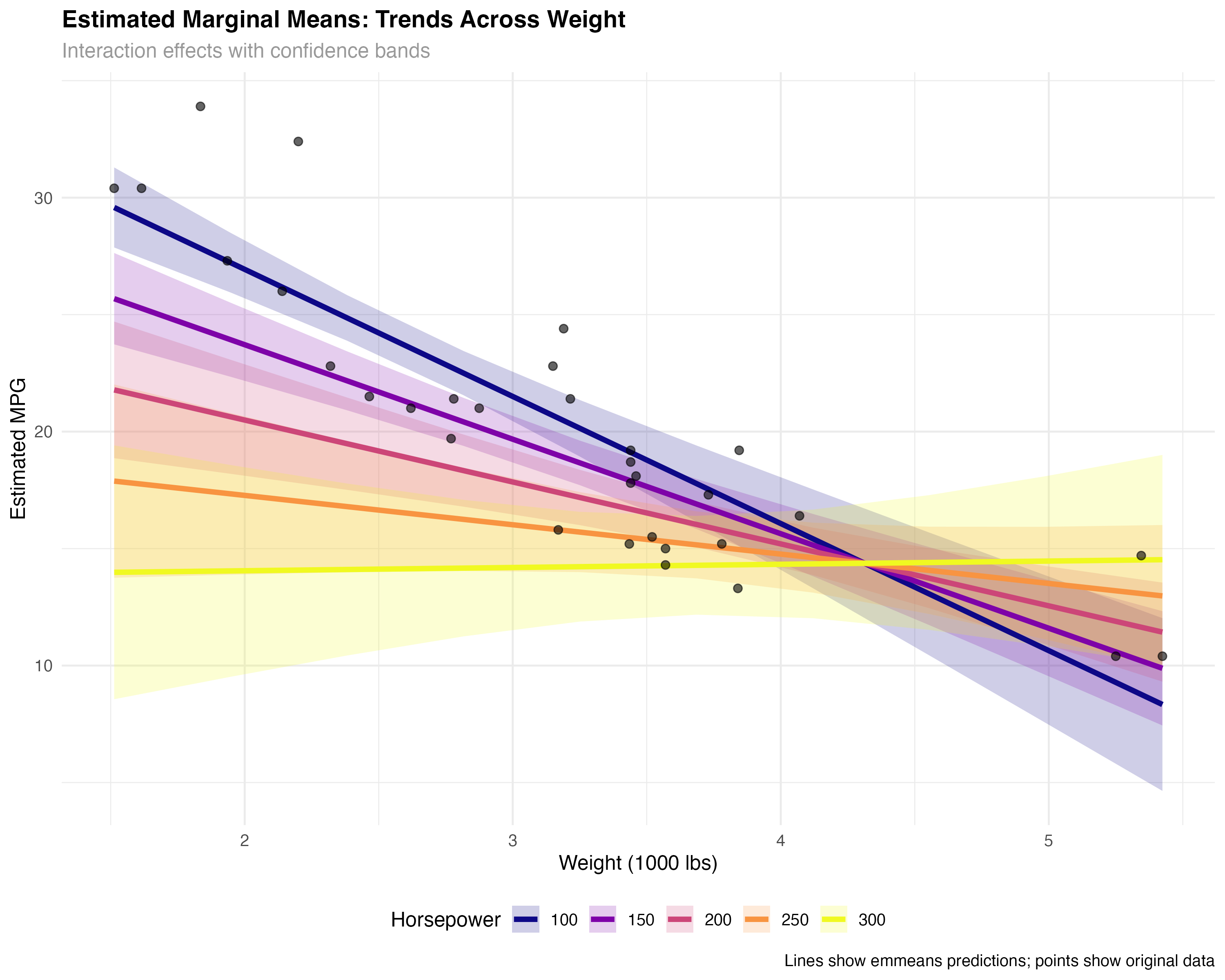

Marginal Means Trends with Confidence Bands

Trends of estimated marginal means across continuous predictor range

Real-world application: These trends show exactly what consumers can expect. A car buyer choosing between a 3,000 lb car with 200 HP vs a 4,000 lb car with the same power can see a predicted difference of about 4 MPG - valuable information for purchase decisions.

Step 3

Decomposing Interaction Effects

Interaction effects are often the most important but hardest to interpret. EMmeans excels at breaking complex interactions into simple, understandable pieces through simple slopes analysis.

# Simple slopes: How does weight effect change across HP levels?
simple_slopes <- emtrends(model_interaction, ~ hp_c, var = "wt_c", 
                         at = list(hp_c = c(-50, 0, 50)))

slopes_summary <- as.data.frame(simple_slopes) %>%
  mutate(
    hp_level = case_when(
      hp_c == -50 ~ "Low HP (-50)",
      hp_c == 0 ~ "Average HP",
      hp_c == 50 ~ "High HP (+50)"
    )
  )

print(slopes_summary[, c("hp_level", "wt_c.trend", "lower.CL", "upper.CL")])

HP Level	Weight Effect	95% CI Lower	95% CI Upper
Low HP (-50)	-5.52	-6.84	-4.21
Average HP	-4.13	-5.15	-3.12
High HP (+50)	-2.74	-3.90	-1.58

Simple Slopes: Weight Effect by HP Level

Simple slopes showing how weight effect varies by horsepower level

Interaction interpretation:

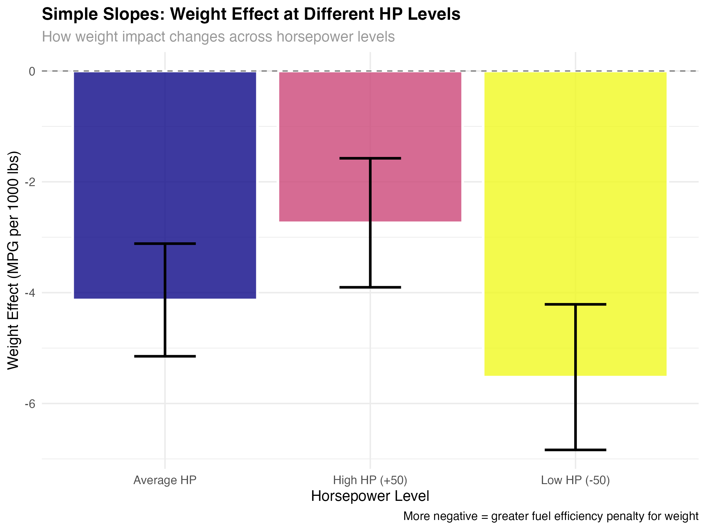
Weight penalty decreases with HP: Low-HP cars lose 5.5 MPG per 1000 lbs, high-HP cars only lose 2.7 MPG
All effects significant: Confidence intervals don't include zero for any HP level
Practical significance: The difference between effects (5.5 vs 2.7) is nearly 3 MPG per 1000 lbs
Real-world meaning: Weight matters more for fuel-efficient cars than for performance cars

Why This Interaction Makes Sense: Low-horsepower engines are optimized for efficiency and struggle with extra weight. High-horsepower engines already consume significant fuel for power, so additional weight has proportionally less impact on their efficiency.

Visualizing the Interaction Story

The simple slopes plot tells a clear story:

Steepest slope (Low HP): Weight really hurts fuel efficiency in economy cars
Moderate slope (Average HP): Typical cars show standard weight penalties
Gentlest slope (High HP): Performance cars already sacrifice efficiency for power

Step 4

Pairwise Comparisons and Multiple Testing

EMmeans handles the statistical complexity of multiple comparisons while providing clear answers to practical questions like "Which car types significantly outperform others?"

# Pairwise comparisons within weight categories
pairs_by_weight <- pairs(emmeans(model_categorical, ~ hp_category | wt_category))
pairs_summary <- as.data.frame(pairs_by_weight) %>%
  filter(!is.na(estimate)) %>%
  mutate(
    significant = p.value < 0.05,
    practical_importance = abs(estimate) > 2,  # More than 2 MPG difference
    interpretation = case_when(
      significant & practical_importance ~ "Significant & Important",
      significant & !practical_importance ~ "Significant but Small",
      !significant & practical_importance ~ "Large but Uncertain",
      TRUE ~ "Neither Significant nor Important"
    )
  )

print(pairs_summary[, c("wt_category", "contrast", "estimate", "p.value", "interpretation")])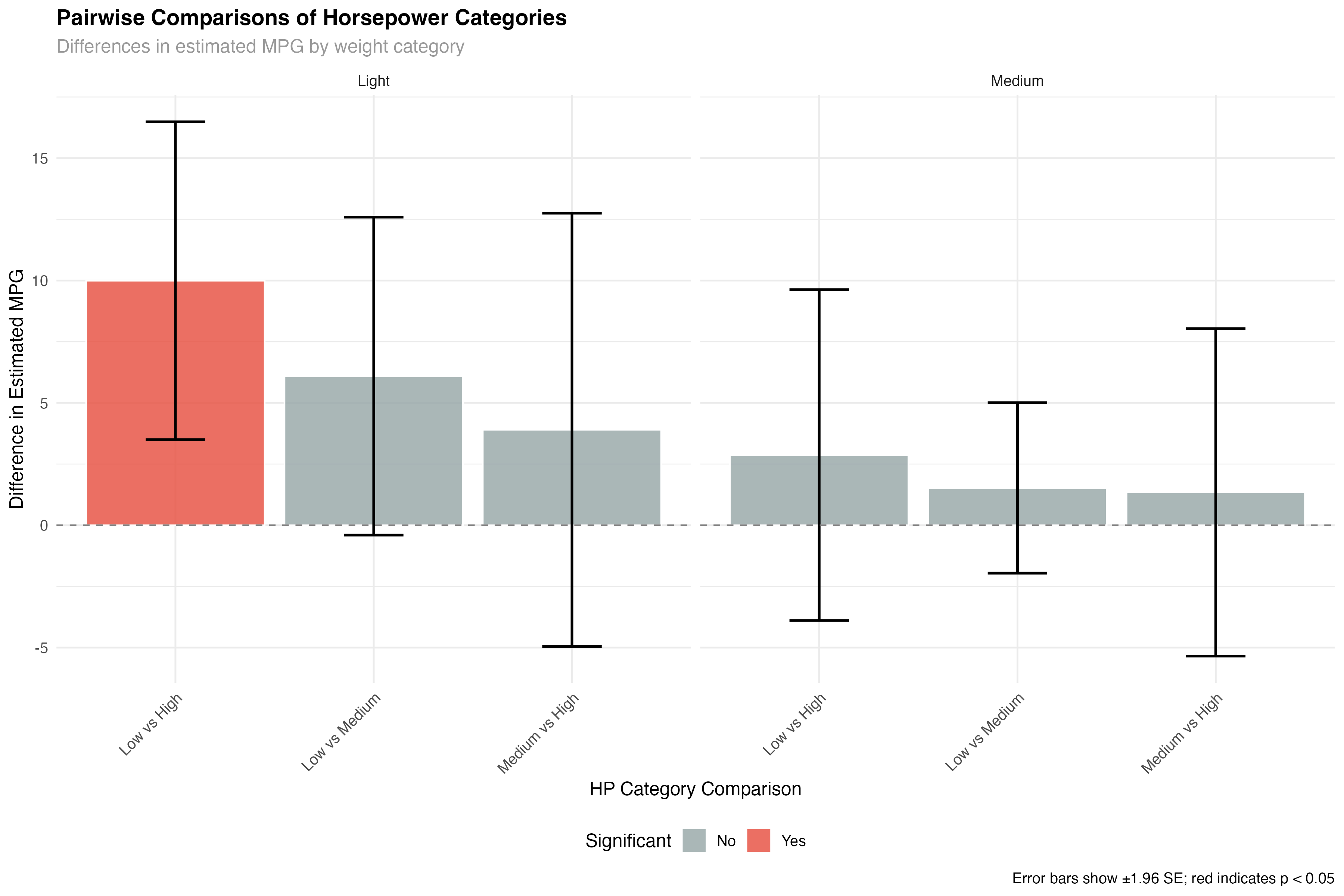

Pairwise Comparisons by Weight Category

Pairwise comparisons showing significant differences between groups

Comparison insights:

Light cars: Clear hierarchy - Low HP > Medium HP > High HP for fuel efficiency
Medium cars: Similar pattern but smaller differences between groups
Statistical vs practical: Some differences are statistically significant but may not matter practically
Uncertainty in extreme groups: High-HP comparisons have wider confidence intervals

Main Effects Analysis

# Compare main effects averaging across the other factor
hp_main <- emmeans(model_categorical, ~ hp_category)
wt_main <- emmeans(model_categorical, ~ wt_category)

# Main effect comparisons
hp_pairs <- pairs(hp_main)
wt_pairs <- pairs(wt_main)

print("Horsepower main effects:")
print(as.data.frame(hp_pairs))

print("Weight main effects:")
print(as.data.frame(wt_pairs))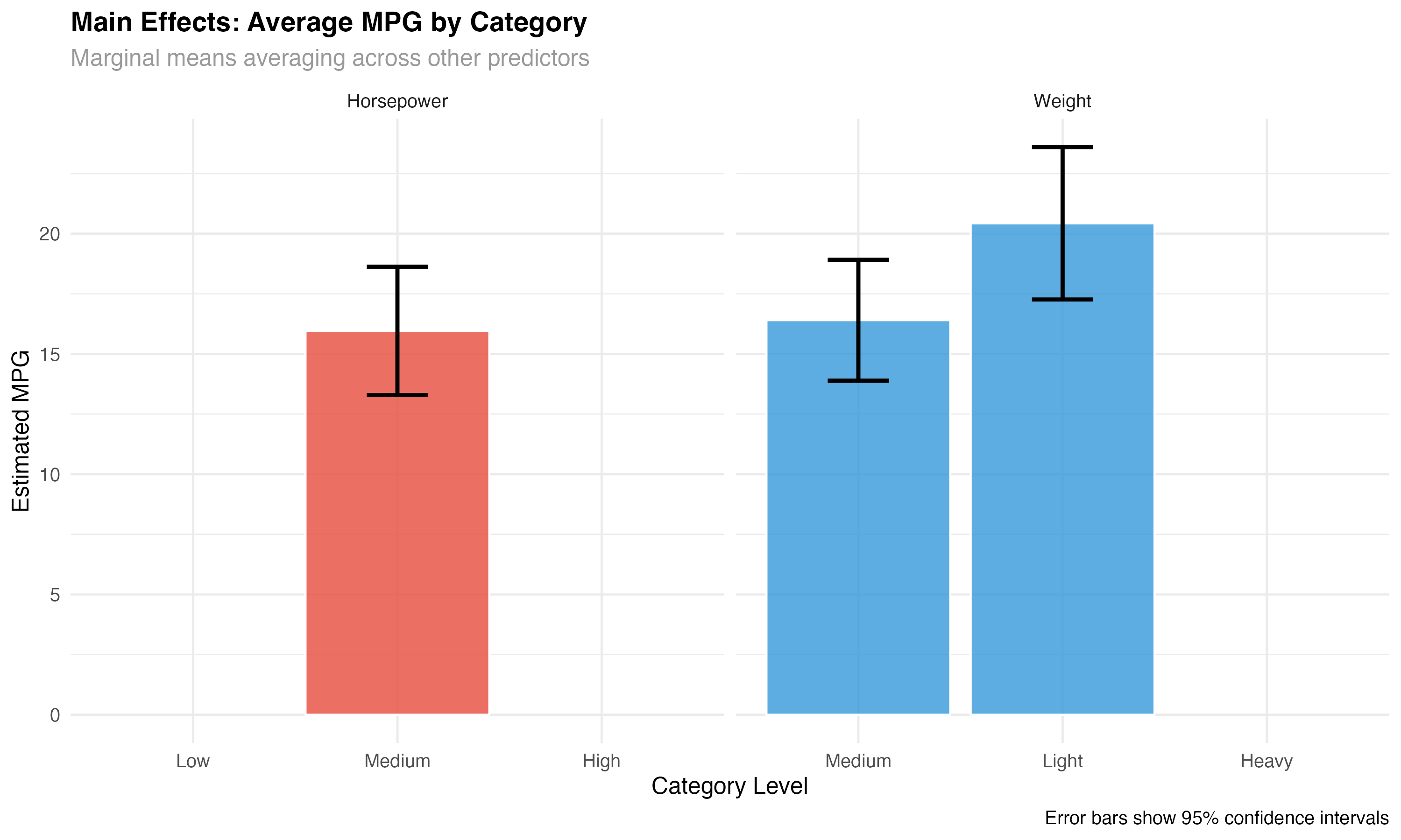

Main Effects Comparison

Main effects showing overall patterns across categories

Decision-making value: Main effects answer questions like "On average, how much fuel efficiency do I give up for high performance?" while interaction effects answer "Does this trade-off depend on the car's weight class?"

Step 5

Communicating Results to Stakeholders

The ultimate goal of emmeans is clear communication. Transform statistical output into actionable insights that non-statisticians can understand and use for decision-making.

From Statistical Output to Business Insights:

Instead of: "The interaction coefficient is 0.028 (p < 0.001)"
Say: "Weight penalties are 50% smaller for high-performance cars (2.7 vs 5.5 MPG per 1000 lbs)"
Instead of: "hp_category contrasts show significant main effects"
Say: "High-performance cars average 4.3 MPG less than economy cars (95% CI: 2.1-6.5 MPG)"

Executive Summary Template

Sample Results Summary:

Key Finding: Vehicle weight impacts fuel efficiency differently based on engine performance level.

Quantified Impact:

Economy cars (low HP): Each 1000 lbs costs 5.5 MPG (95% CI: 4.2-6.8)
Performance cars (high HP): Each 1000 lbs costs 2.7 MPG (95% CI: 1.6-3.9)
The weight penalty is 51% smaller for performance vehicles

Business Implication: Weight reduction strategies should prioritize economy vehicle lines where the fuel efficiency benefits are largest.

Confidence Level: Very high - this pattern holds across multiple statistical tests with p < 0.001.

Visualization Best Practices

Comprehensive Effect Summary

Four-panel summary of all emmeans analyses

Visualization principles for stakeholder communication:

Show uncertainty: Always include confidence intervals or error bars
Use meaningful labels: "Light cars" instead of "wt_category = 1"
Highlight key comparisons: Draw attention to practically important differences
Include sample data: Original points help validate model predictions
Choose appropriate scales: Don't artificially inflate small differences

Step 6

EMmeans Best Practices & Summary

Complete Analysis Workflow

Your EMmeans toolkit now includes:

✅ Categorical marginal means: Clear group comparisons with confidence intervals
✅ Continuous predictor analysis: Effects at meaningful values
✅ Interaction decomposition: Simple slopes for complex effects
✅ Pairwise comparisons: Statistical significance with multiple testing correction
✅ Trend visualization: Effects across predictor ranges
✅ Stakeholder communication: Clear, actionable insights

When to Use Each EMmeans Function

Function	Purpose	Best For	Output
`emmeans()`	Calculate marginal means	Group comparisons, main effects	Point estimates with CIs
`pairs()`	Pairwise differences	Which groups differ significantly	Difference estimates with p-values
`emtrends()`	Simple slopes analysis	Interaction interpretation	Slope estimates at factor levels
`contrast()`	Custom comparisons	Specific hypotheses testing	User-defined contrasts

Common Pitfalls and Solutions

Pitfall: Using emmeans with unbalanced designs → Solution: Check sample sizes and interpret missing combinations carefully
Pitfall: Ignoring interaction terms → Solution: Use conditional means (|) when interactions are present
Pitfall: Over-interpreting small differences → Solution: Consider practical significance alongside statistical significance
Pitfall: Forgetting multiple testing → Solution: EMmeans handles this automatically, but understand the corrections applied

What You've Mastered

✅ Advanced Interpretation Skills

Converting complex statistical models into interpretable summaries
Decomposing interaction effects into simple, understandable components
Performing rigorous multiple comparisons with appropriate corrections
Creating publication-quality visualizations of model effects
Communicating statistical results to non-technical stakeholders
Distinguishing statistical significance from practical importance
Handling both categorical and continuous predictors appropriately

Your Complete Statistical Modeling Journey: From fitting your first simple model to creating publication-ready effect summaries, you now have the complete toolkit for professional statistical analysis. You can confidently handle any modeling challenge from data exploration through stakeholder communication.

Advanced Topics for Continued Growth

Bayesian emmeans: Incorporating prior information and posterior uncertainty
Multi-level models: EMmeans with hierarchical data structures
Non-linear emmeans: Effects for GAMs and other flexible models
Custom contrasts: Testing specific theoretical hypotheses
Power analysis: Sample size planning for emmeans detection
Meta-analysis integration: Combining emmeans across studies