Mastering the Broom Ecosystem: Tidy Model Workflows in R

🎯 Learning Objectives

Master the core broom functions: tidy(), glance(), and augment()
Compare model outputs across different statistical approaches
Implement efficient batch processing workflows for multiple models
Create automated model reporting pipelines
Visualize coefficient evolution and model comparison metrics
Apply tidy modeling principles to real-world data analysis

📊

The Broom Philosophy

Transforming messy model outputs into tidy data

🧹 What is Broom?

The broom package provides a consistent framework for converting statistical model outputs into tidy data frames. Instead of dealing with inconsistent list structures and messy model summaries, broom standardizes the process of extracting key information from any statistical model.

tidy() - Coefficient Information

Extracts coefficient estimates
Provides standard errors and p-values
Includes confidence intervals
Consistent format across model types
Compatible with tidyverse workflows

glance() - Model Statistics

Model fit statistics (R², AIC, BIC)
Sample size and degrees of freedom
Model comparison metrics
One row per model summary
Ideal for model selection workflows

augment() - Observation-Level Data

Fitted values and residuals
Leverage and influence measures
Prediction intervals
Original data with model outputs
Essential for model diagnostics

⚙️

Core Broom Functions

Essential tools for tidy modeling workflows

Setting Up the Broom Ecosystem R

library(tidyverse)
library(glmmTMB)
library(broom)
library(broom.mixed)
library(ggplot2)
library(patchwork)

# Enhanced dataset for comprehensive broom demonstration
data(mtcars)
mtcars_enhanced <- mtcars %>%
  mutate(
    # Factor variables for categorical analysis
    transmission = factor(am, levels = c(0, 1), labels = c("Automatic", "Manual")),
    cyl_factor = factor(cyl, levels = c(4, 6, 8), labels = c("4-cyl", "6-cyl", "8-cyl")),
    vs_factor = factor(vs, levels = c(0, 1), labels = c("V-shaped", "Straight")),
    # Scaled continuous predictors
    wt_scaled = scale(wt)[,1],
    hp_scaled = scale(hp)[,1],
    # Binary outcome for logistic regression demo
    high_mpg = factor(ifelse(mpg > median(mpg), "High", "Low"))
  )

# Fit multiple model types for broom demonstration
model_linear <- lm(mpg ~ wt_scaled + hp_scaled + transmission, data = mtcars_enhanced)
model_glmm <- glmmTMB(mpg ~ wt_scaled * hp_scaled + (1|cyl_factor), data = mtcars_enhanced)
model_logistic <- glm(high_mpg ~ wt_scaled, family = binomial, data = mtcars_enhanced)

💡 Key Design Principle

The broom ecosystem follows the principle of consistent interfaces. Whether you're working with linear models, mixed-effects models, or machine learning algorithms, the same three functions (tidy, glance, augment) provide predictable outputs that integrate seamlessly with tidyverse workflows.

🔍

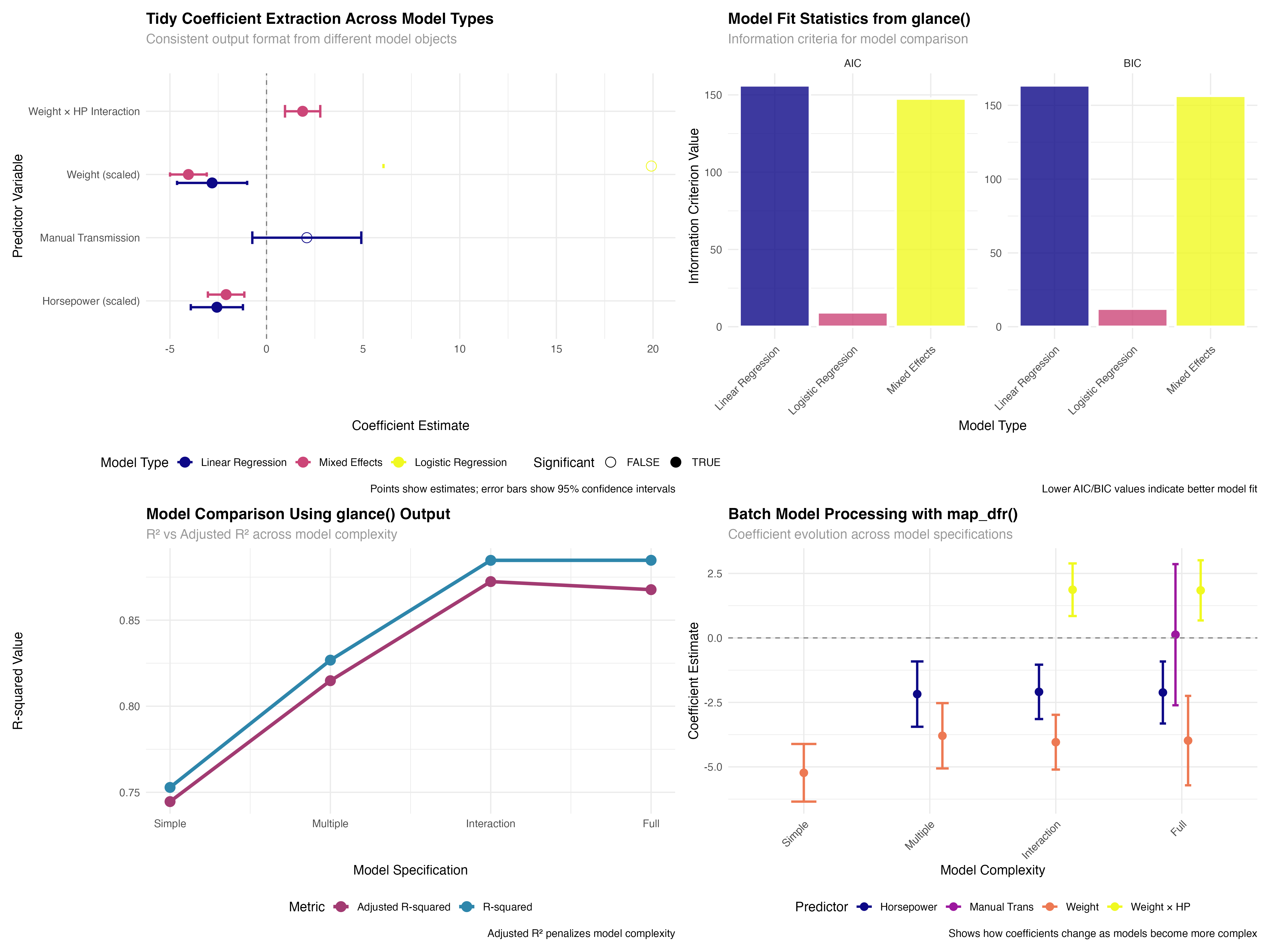
Comparing Model Types with Broom

Consistent coefficient extraction across different approaches

Extracting Coefficients with tidy() R

# Basic broom functions comparison
# tidy() - Extract coefficient information
tidy_linear <- tidy(model_linear, conf.int = TRUE)
tidy_glmm <- tidy(model_glmm, conf.int = TRUE)
tidy_logistic <- tidy(model_logistic, conf.int = TRUE)

# Combine results for comparison
tidy_comparison <- bind_rows(
  tidy_linear %>% mutate(model_type = "Linear Regression"),
  tidy_glmm %>% filter(effect == "fixed") %>% mutate(model_type = "Mixed Effects"),
  tidy_logistic %>% mutate(model_type = "Logistic Regression")
) %>%
  filter(term != "(Intercept)") %>%
  mutate(
    term_clean = case_when(
      term == "wt_scaled" ~ "Weight (scaled)",
      term == "hp_scaled" ~ "Horsepower (scaled)", 
      term == "transmissionManual" ~ "Manual Transmission",
      term == "wt_scaled:hp_scaled" ~ "Weight × HP Interaction",
      TRUE ~ term
    ),
    significant = p.value < 0.05,
    model_type = factor(model_type, levels = c("Linear Regression", "Mixed Effects", "Logistic Regression"))
  )

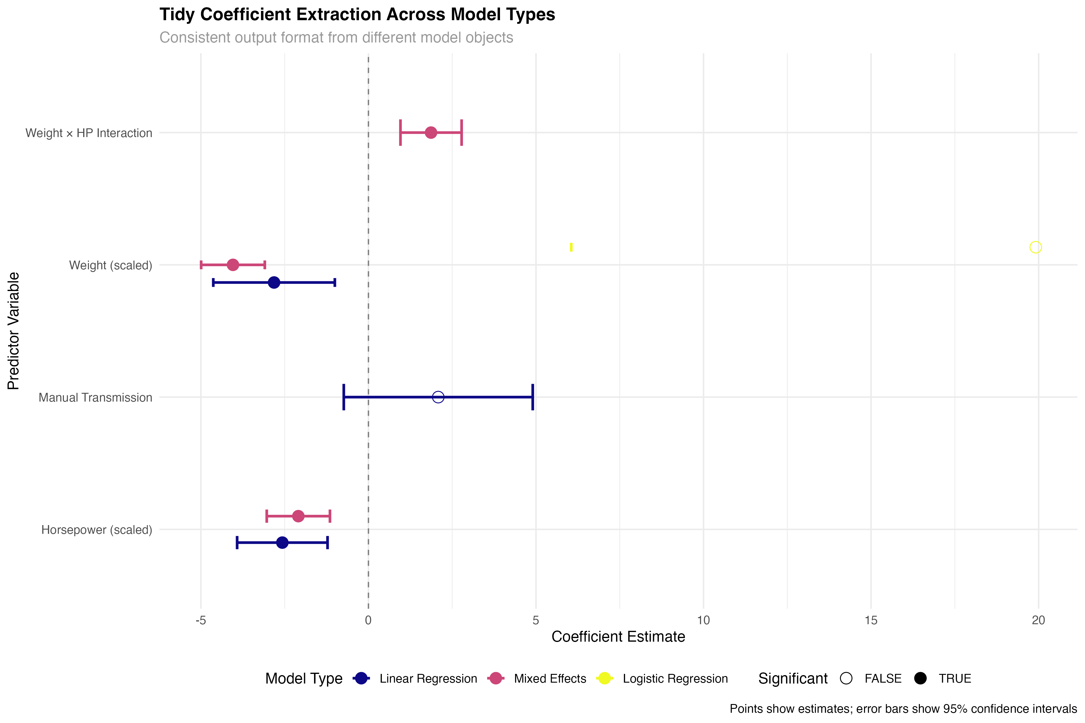
Figure 1: Coefficient extraction across model types using tidy(). Note how broom provides consistent output formats regardless of the underlying model structure, enabling direct comparison of effect sizes and significance across different statistical approaches.

✅ Broom Advantage

Notice how the same tidy() function works seamlessly across linear models, mixed-effects models, and generalized linear models. This consistency eliminates the need to remember different extraction methods for different model types, dramatically simplifying comparative analyses.

📈

Model Fit Statistics with glance()

Standardized model comparison metrics

Extracting Model Statistics R

# glance() - Extract model-level statistics  
glance_linear <- glance(model_linear)
glance_glmm <- glance(model_glmm)
glance_logistic <- glance(model_logistic)

# Create comparison of key metrics
glance_comparison <- bind_rows(
  glance_linear %>% select(r.squared, adj.r.squared, AIC, BIC, nobs) %>% 
    mutate(model_type = "Linear Regression"),
  glance_glmm %>% select(r.squared = sigma, adj.r.squared = sigma, AIC, BIC, nobs) %>% 
    mutate(model_type = "Mixed Effects"),
  glance_logistic %>% select(r.squared = deviance, adj.r.squared = null.deviance, AIC, BIC, nobs) %>% 
    mutate(model_type = "Logistic Regression")
) %>%
  select(model_type, AIC, BIC, nobs) %>%
  pivot_longer(cols = c(AIC, BIC), names_to = "metric", values_to = "value")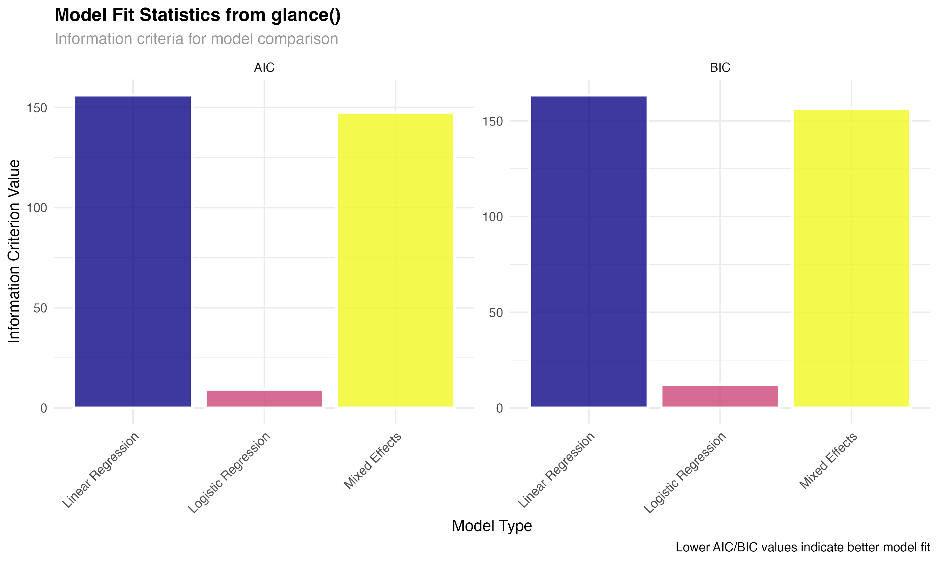

Figure 2: Model fit statistics extracted using glance(). Information criteria (AIC, BIC) provide standardized metrics for comparing models of different types, with lower values indicating better fit while accounting for model complexity.

Extract Statistics

Use glance() to obtain model-level statistics including fit measures, information criteria, and sample sizes.

Standardize Metrics

Convert different model-specific statistics into comparable formats using consistent naming conventions.

Compare Models

Leverage information criteria and fit statistics to make informed decisions about model selection and adequacy.

🔧

Diagnostic Analysis with augment()

Model validation through observation-level statistics

Adding Model Outputs to Data R

# augment() - Add fitted values and residuals
augment_linear <- augment(model_linear)
augment_glmm <- augment(model_glmm)

# Focus on linear model for residual analysis
residual_data <- augment_linear %>% 
  mutate(model_type = "Linear Regression") %>%
  filter(!is.na(.resid))

# Create diagnostic plot
ggplot(residual_data, aes(x = .fitted, y = .resid)) +
  geom_point(alpha = 0.7, size = 2, color = "#2E86AB") +
  geom_smooth(se = FALSE, linewidth = 1, method = "loess", color = "#A23B72") +
  geom_hline(yintercept = 0, linetype = "dashed", color = "gray50") +
  labs(
    title = "Residual Analysis from augment()",
    subtitle = "Model diagnostics using standardized broom output",
    x = "Fitted Values",
    y = "Residuals"
  )

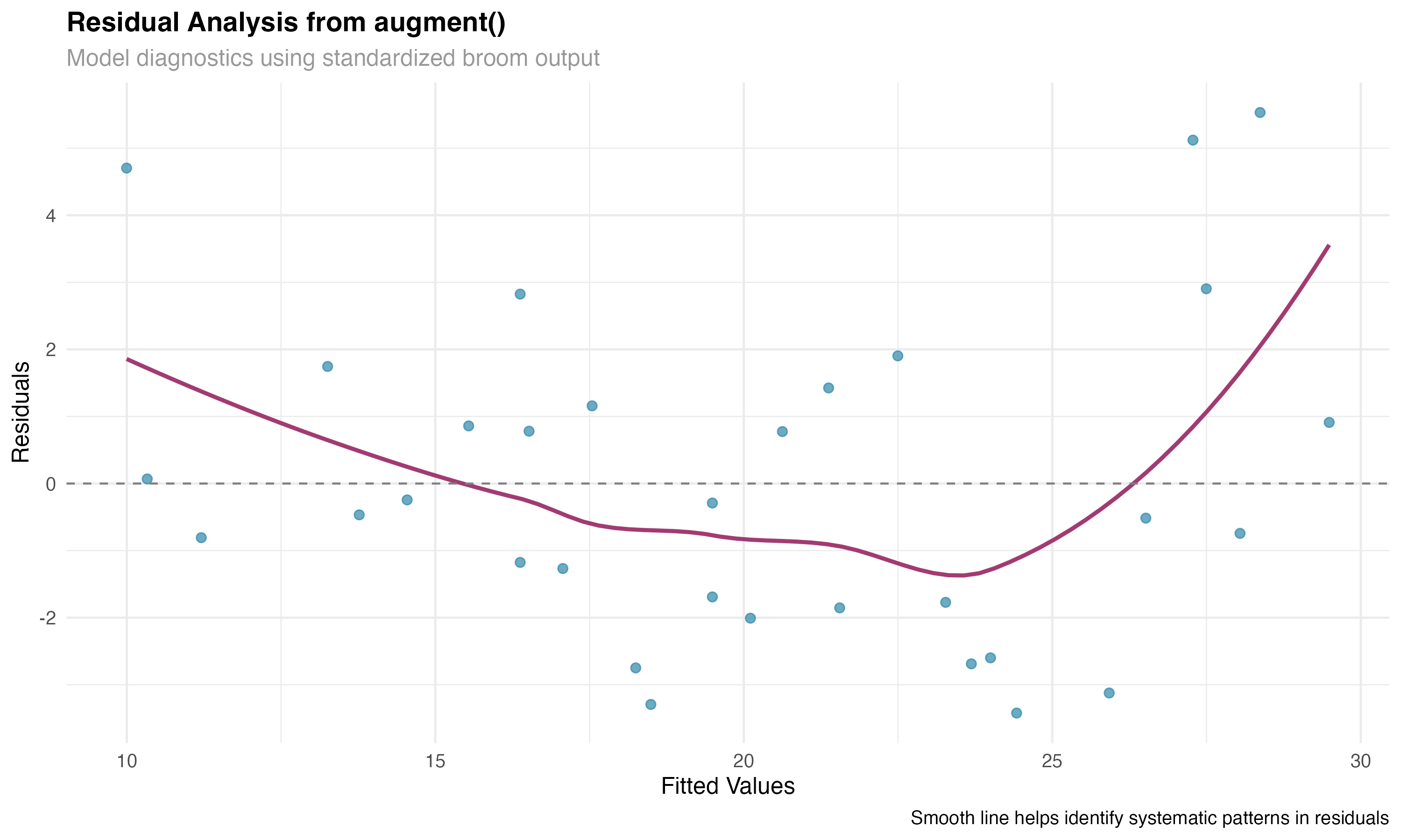
Figure 3: Residual analysis using augment() output. The standardized format makes it easy to create diagnostic plots and assess model assumptions across different model types.

⚠️ Model Validation

The augment() function is essential for model validation. By adding fitted values, residuals, and influence measures to your original data, you can easily create comprehensive diagnostic plots and identify potential problems with model assumptions or outlying observations.

⚡

Batch Processing Workflows

Efficient analysis of multiple models simultaneously

Processing Multiple Models R

# Model comparison workflow using multiple models
models_list <- list(
  "Simple" = lm(mpg ~ wt_scaled, data = mtcars_enhanced),
  "Multiple" = lm(mpg ~ wt_scaled + hp_scaled, data = mtcars_enhanced),
  "Interaction" = lm(mpg ~ wt_scaled * hp_scaled, data = mtcars_enhanced),
  "Full" = lm(mpg ~ wt_scaled * hp_scaled + transmission, data = mtcars_enhanced)
)

# Extract glance statistics for all models using map_dfr
model_stats <- map_dfr(models_list, glance, .id = "model") %>%
  mutate(
    model = factor(model, levels = c("Simple", "Multiple", "Interaction", "Full")),
    complexity = 1:4,
    parameters = c(2, 3, 4, 5)  # Including intercept
  )

# Batch processing workflow
# Process multiple models efficiently with broom
all_tidy <- map_dfr(models_list, tidy, conf.int = TRUE, .id = "model")
all_glance <- map_dfr(models_list, glance, .id = "model")
all_augment <- map_dfr(models_list, augment, .id = "model")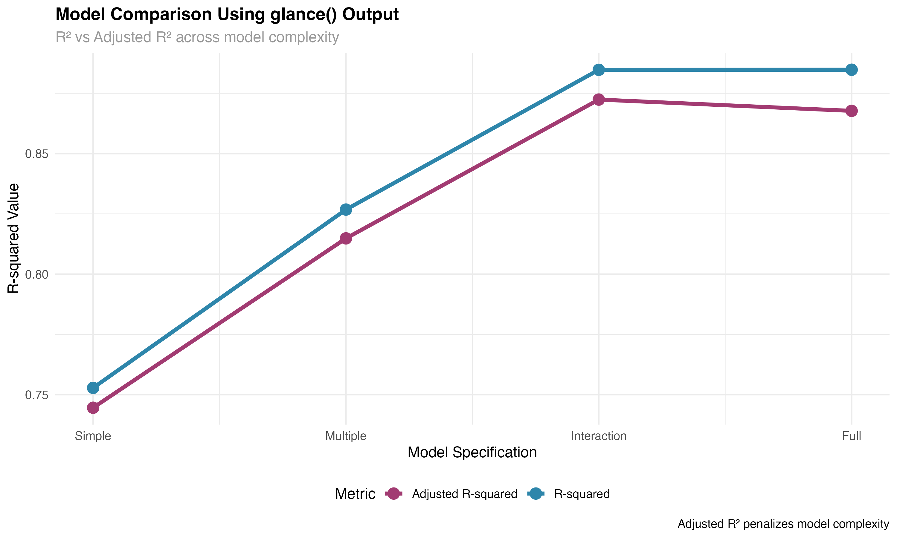

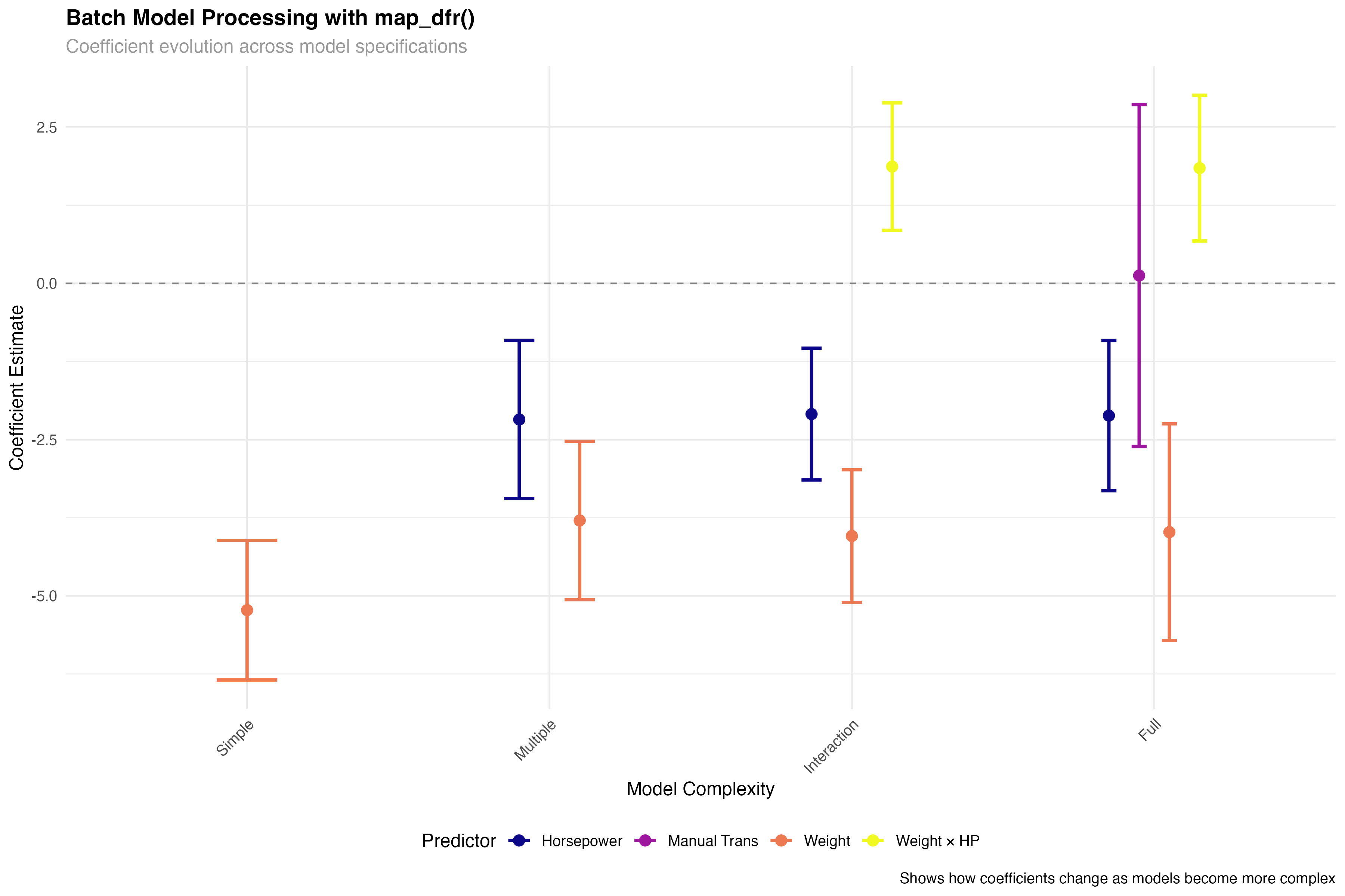
Figure 4: Model comparison using batch processing with map_dfr(). This approach efficiently extracts statistics from multiple models and visualizes the trade-off between model complexity and goodness-of-fit.

Figure 5: Coefficient evolution across model specifications. Batch processing allows us to track how parameter estimates change as we add complexity, providing insights into model stability and predictor relationships.

🚀 Efficiency Gains

Batch processing with broom and purrr's map functions enables powerful workflow automation. Instead of manually extracting statistics from each model, you can process dozens of models simultaneously, making large-scale model comparison and selection feasible and efficient.

🤖

Automated Model Reporting

Creating reproducible analysis pipelines

Custom Model Summary Function R

# Custom broom workflow function
create_model_summary <- function(model, model_name) {
  # Use broom functions to extract key information
  tidy_results <- tidy(model, conf.int = TRUE)
  glance_results <- glance(model)
  
  # Calculate summary metrics
  n_predictors <- nrow(tidy_results) - 1  # Exclude intercept
  n_significant <- sum(tidy_results$p.value[-1] < 0.05, na.rm = TRUE)  # Exclude intercept
  max_effect <- max(abs(tidy_results$estimate[-1]), na.rm = TRUE)
  
  # Return structured summary
  tibble(
    model_name = model_name,
    n_predictors = n_predictors,
    n_significant = n_significant,
    r_squared = round(glance_results$r.squared, 3),
    adj_r_squared = round(glance_results$adj.r.squared, 3),
    aic = round(glance_results$AIC, 1),
    max_effect = round(max_effect, 2)
  )
}

# Apply to all models
model_summaries <- map2_dfr(models_list, names(models_list), create_model_summary)

📊 Model Summary Dashboard

# A tibble: 4 × 7
  model_name   n_predictors n_significant r_squared adj_r_squared   aic max_effect
  <chr>               <dbl>         <int>     <dbl>         <dbl> <dbl>      <dbl>
1 Simple                  1             1     0.753         0.745  166        5.23
2 Multiple                2             2     0.827         0.815  157.       3.79
3 Interaction             3             3     0.885         0.872  146.       4.04
4 Full                    4             3     0.885         0.868  148.       3.98

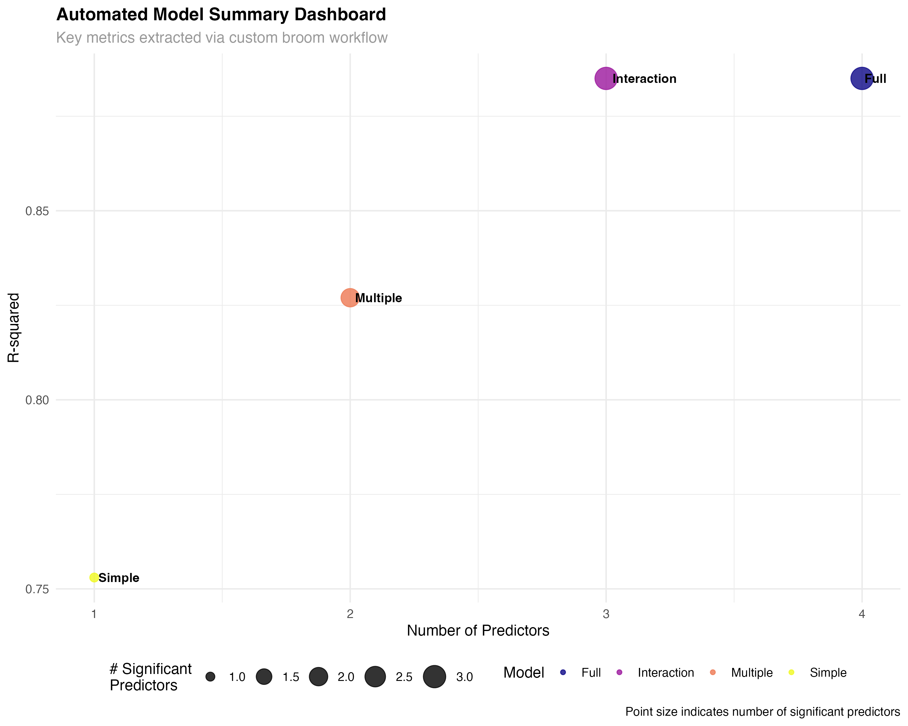
Figure 6: Automated model reporting dashboard. This visualization combines key metrics from tidy() and glance() outputs to provide a comprehensive overview of model performance, with point size indicating the number of significant predictors.

✨ Reproducible Workflows

Custom functions that leverage broom's consistent interfaces enable fully reproducible analysis pipelines. These automated workflows can be easily adapted to different datasets and model types, ensuring consistency and efficiency across projects.

🎨

Enhanced Visualizations

Advanced coefficient plots and model comparisons

Enhanced Coefficient Visualization R

# Tidy coefficient plot with enhanced formatting
enhanced_coef_plot <- all_tidy %>%
  filter(term != "(Intercept)", model %in% c("Multiple", "Interaction", "Full")) %>%
  mutate(
    term_clean = case_when(
      term == "wt_scaled" ~ "Weight (scaled)",
      term == "hp_scaled" ~ "Horsepower (scaled)",
      term == "transmissionManual" ~ "Manual Transmission", 
      term == "wt_scaled:hp_scaled" ~ "Weight × HP Interaction",
      TRUE ~ term
    ),
    significant = p.value < 0.05,
    effect_size = case_when(
      abs(estimate) < 1 ~ "Small",
      abs(estimate) < 3 ~ "Medium",
      TRUE ~ "Large"
    ),
    model = factor(model, levels = c("Multiple", "Interaction", "Full"))
  ) %>%
  ggplot(aes(x = reorder(term_clean, estimate), y = estimate)) +
  geom_hline(yintercept = 0, linetype = "dashed", color = "gray50") +
  geom_errorbar(aes(ymin = conf.low, ymax = conf.high, color = significant), 
                width = 0.3, linewidth = 1) +
  geom_point(aes(color = significant, size = effect_size), alpha = 0.8) +
  facet_wrap(~ model, ncol = 1) +
  scale_color_manual(values = c("FALSE" = "#95a5a6", "TRUE" = "#e74c3c"),
                     name = "Significant") +
  scale_size_manual(values = c("Small" = 2, "Medium" = 3, "Large" = 4),
                    name = "Effect Size") +
  coord_flip()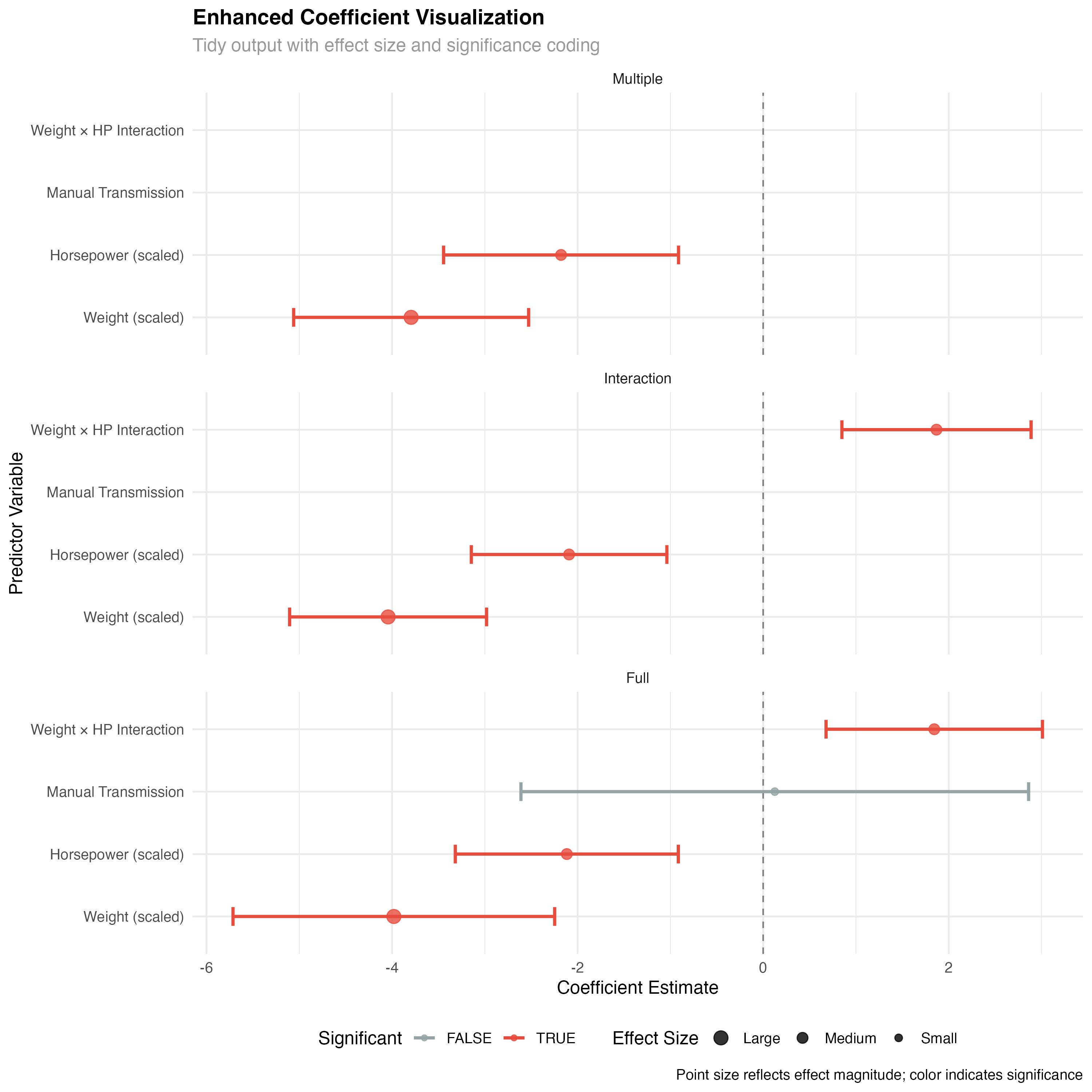

Figure 7: Enhanced coefficient visualization with effect size and significance coding. This plot demonstrates how broom's tidy output can be extended with custom categorical variables to create rich, informative visualizations.

Figure 8: Comprehensive broom workflow visualization. This panel combines coefficient comparison, model fit statistics, complexity analysis, and batch processing results to demonstrate the full power of the broom ecosystem for tidy modeling workflows.

🏆 Practice Exercise: Build Your Own Broom Pipeline

Apply the broom ecosystem to your own data analysis:

Load a dataset with multiple potential predictors
Fit 3-4 competing models with different complexity levels
Use map_dfr() to extract tidy(), glance(), and augment() results
Create a model comparison visualization
Build an automated reporting function
Generate diagnostic plots using augment() output

🎓

Key Takeaways

Essential principles for mastering broom workflows

Consistency is Power

The broom ecosystem provides consistent interfaces across all model types, dramatically simplifying comparative analyses and enabling standardized workflows.

Batch Processing Efficiency

Combine broom with purrr's mapping functions to process multiple models simultaneously, enabling large-scale model comparison and selection.

Automated Reporting

Build custom functions that leverage broom's standardized outputs to create reproducible analysis pipelines and automated model summaries.

Integration with Tidyverse

Broom outputs are designed to work seamlessly with dplyr, ggplot2, and other tidyverse tools, enabling powerful data manipulation and visualization workflows.